Draw a bifurcation diagram over fishing effort

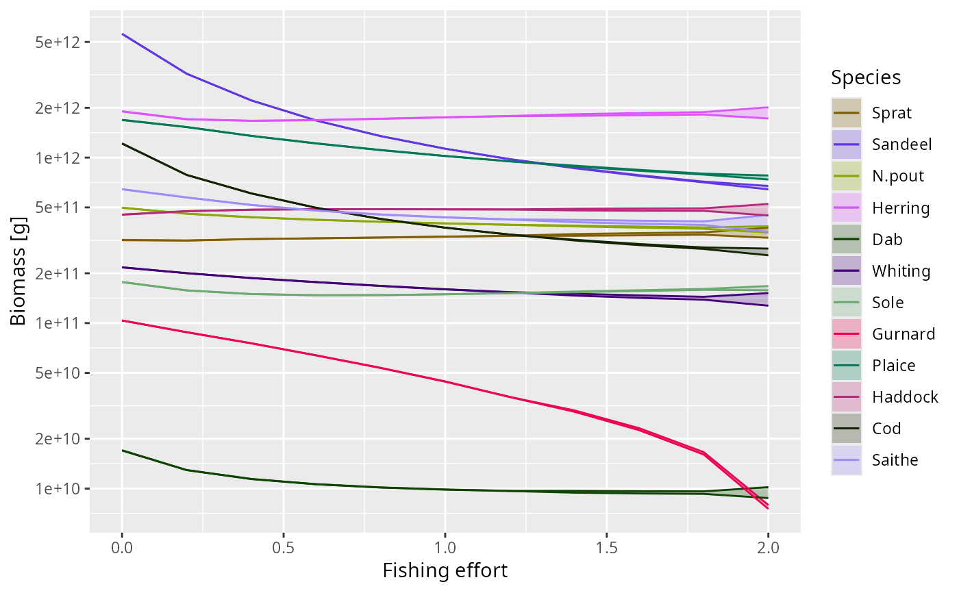
Sweeps the fishing effort over a range of values and, for each value, runs the full dynamics to their attractor and records the long-term range of a summary quantity (biomass by default). The result is a bifurcation diagram with fishing effort on the x-axis.

For each effort value the attractor is found in two stages. First projectToSteady() runs the dynamics until they settle, stopping early once it detects a stable steady state or a limit cycle and reporting which via its "convergence" attribute. Then the settled state is projected forward once more with project() over a short sampling window — one full period for a limit cycle, or a few years otherwise — and the minimum and maximum of the chosen quantity over that window are taken as the attractor envelope.

For a stable steady state the minimum and maximum coincide and the species is drawn as a single line; once the dynamics settle onto a limit cycle the two separate and the species is drawn as a shaded band between them. The onset of the band therefore marks the Hopf bifurcation (see vignette("dynamic_stability")).

By default the sweep uses continuation: the projection at each effort value starts from the attractor reached at the previous value rather than from the original state. This shortens the transient and keeps the sweep on a single branch of the attractor. Because it follows one branch, the diagram can look different for an increasing versus a decreasing effort sequence if the model has coexisting attractors (hysteresis); pass a decreasing effort vector to trace the other direction.

Usage

plotBifurcation(
  params,
  effort = seq(0, 2, length.out = 21),
  species = NULL,
  value = c("biomass", "yield", "ssb"),
  t_max = 100,
  t_sample = NULL,
  t_sample_default = 10,
  t_save = 0.25,
  tol = 0.01,
  amplitude_tol = 0.01,
  extinction_threshold = 1e-06,
  continuation = TRUE,
  return_data = FALSE,
  progress_bar = TRUE,
  ytrans = "log10"
)

Arguments

params

A MizerParams object.

effort

A numeric vector of fishing effort values for the x-axis. The same effort is applied to every gear (as in project(effort = value)). Default seq(0, 2, length.out = 21).

species

The species to include. By default all target species. A vector of species names or indices, as for other mizer plotting functions.

value

The quantity for the y-axis, one of "biomass" (default), "yield" or "ssb", computed with getBiomass(), getYield() or getSSB() respectively.

t_max

The maximum number of years to run the settling stage (projectToSteady()) at each effort value.

t_sample

The length in years of the window over which the settled attractor is sampled to measure the envelope. If NULL (default) it is chosen automatically: one full period for a detected limit cycle, or t_sample_default years otherwise.

t_sample_default

The sampling window used when no limit-cycle period is available (a stable or non-converged run). Default 10.

t_save

The interval at which the sampling window is saved, controlling how finely the cycle envelope is resolved. Default 0.25.

tol

Convergence tolerance for the settling stage, passed to projectToSteady(). Tighter (smaller) values settle the stable branch more fully, giving cleaner single lines below the bifurcation at the cost of longer runs. Default 0.01.

amplitude_tol

The minimum relative biomass amplitude for a run to be classified as a limit cycle, passed to projectToSteady(). Default 0.01.

extinction_threshold

The relative reproduction collapse below which a species is treated as extinct, passed to projectToSteady(). Default 1e-6.

continuation

If TRUE (default) each settling run warm-starts from the attractor of the previous effort value.

return_data

If TRUE the data frame underlying the plot is returned instead of the plot. Default FALSE.

progress_bar

If TRUE (default) a text progress bar is shown while the effort values are swept.

ytrans

Transformation for the y-axis, "log10" (default) or "identity".

Value

A ggplot2 object, or a data frame with columns Effort, Species, ymin, ymax and type (the attractor type reported by projectToSteady()) if return_data = TRUE.

See also

getStability(), projectToSteady(), plotBiomass()

Other plotting functions: addPlot(), animate(), plot, plot2(), plotBiomass(), plotCDF(), plotCDF2(), plotDiet(), plotFMort(), plotFeedingLevel(), plotGrowthCurves(), plotMizerParams, plotMizerSim, plotPredMort(), plotRelative(), plotSpectra(), plotSpectra2(), plotSpectraRelative(), plotYield(), plotYieldGear(), plotting_functions

Examples

# \donttest{
plotBifurcation(NS_params, effort = seq(0, 2, length.out = 11))
#> 
  |                                                                            
  |                                                                      |   0%
  |                                                                            
  |======                                                                |   9%
  |                                                                            
  |=============                                                         |  18%
  |                                                                            
  |===================                                                   |  27%
  |                                                                            
  |=========================                                             |  36%
  |                                                                            
  |================================                                      |  45%
  |                                                                            
  |======================================                                |  55%
  |                                                                            
  |=============================================                         |  64%
  |                                                                            
  |===================================================                   |  73%
  |                                                                            
  |=========================================================             |  82%
  |                                                                            
  |================================================================      |  91%
  |                                                                            
  |======================================================================| 100%

# }