Plot the relative difference between two spectra

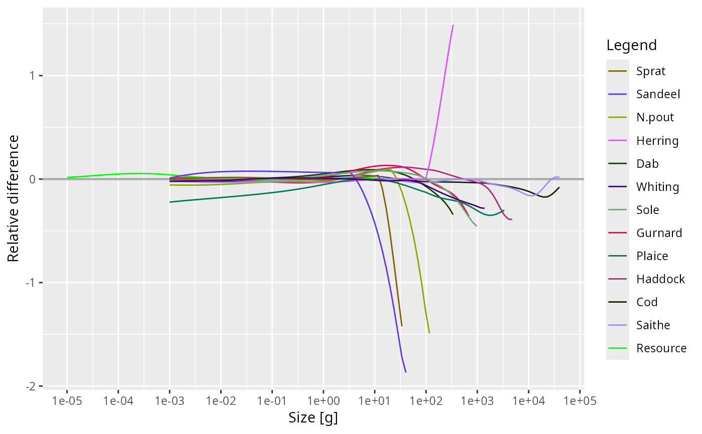
plotSpectraRelative() plots the difference between the spectra relative to their average. If we denote the number density from the first object as \(N_1(w)\) and that from the second object as \(N_2(w)\), then this plot shows $$2 (N_2(w) - N_1(w)) / (N_2(w) + N_1(w)).$$

Usage

plotSpectraRelative(object1, object2, log_x = TRUE, ylim = c(NA, NA), ...)

plotlySpectraRelative(object1, object2, log_x = TRUE, ylim = c(NA, NA), ...)

Arguments

object1

First MizerParams or MizerSim object.

object2

Second MizerParams or MizerSim object.

log_x

If TRUE (default), use a log10 x-axis.

ylim

A numeric vector of length two providing lower and upper limits for the relative difference (y) axis. Use NA to refer to the existing minimum or maximum.

...

Arguments passed to plotSpectra() for preparing the spectra data, for example species, time_range, wlim, resource, background or total.

Value

A ggplot2 object.

Details

The individual spectra are calculated by plotSpectra(), to which all additional arguments are passed. For example, you can determine a time range over which to average simulation results via time_range. See plotSpectra() for more options.

Note that it does not matter whether the relative difference is calculated for number density, biomass density, or biomass density in log weight, because the factors of \(w\) by which the densities differ cancel out in the relative difference.

See also

Other plotting functions: addPlot(), animate.ArrayTimeBySpeciesBySize(), plot, plot2(), plotBiomass(), plotCDF(), plotCDF2(), plotDiet(), plotFMort(), plotFeedingLevel(), plotGrowthCurves(), plotMizerParams, plotMizerSim, plotPredMort(), plotRelative(), plotSpectra(), plotSpectra2(), plotYield(), plotYieldGear(), plotting_functions

Examples

# \donttest{
sim1 <- project(NS_params, t_max = 10, progress_bar = FALSE)
sim2 <- project(NS_params, effort = 0.5, t_max = 10, progress_bar = FALSE)
plotSpectraRelative(sim1, sim2)

# }