The Numerical Scheme used in Mizer

In this vignette we explain the numerical scheme used in mizer. We will not go into the details of the model itself, which is described in the model description vignette. We will focus on how the model is discretised and how the resulting difference equations are solved.

The weight grid

The model dynamics are described by partial differential equations (PDEs) for the consumer number density \(N(w)\) of each species and the resource number density \(N_R(w)\). These depend on the individual weight \(w\). To solve these equations numerically, we discretise the weight axis. In this vignette we suppress the species index and write the equations for one species; the same scheme is applied to each species.

We choose a grid of weights \(w_1, w_2, \ldots, w_K\). The grid is logarithmically spaced, meaning that the ratio of consecutive weights is constant: \[ w_{j+1} / w_j = 10^{\Delta x} = \text{const}. \tag{1}\] The logarithmic spacing is chosen because the weights of fish span many orders of magnitude, from milligrams to megagrams.

This grid defines a set of bins. The \(j\)-th bin is the interval \([w_j, w_{j+1})\). The width of the \(j\)-th bin is \[ \Delta w_j = w_{j+1} - w_j = w_j (10^{\Delta x} - 1). \tag{2}\] Note that \(\Delta w_j\) increases with \(w_j\), which is appropriate for a logarithmic grid.

In the finite-volume scheme used by mizer, the discrete value \(N_j\) represents the average of the number density \(N(w)\) over the \(j\)-th bin, \[ N_j = \frac{1}{\Delta w_j} \int_{w_j}^{w_{j+1}} N(w)\, dw, \tag{3}\] so that the number of individuals in the \(j\)-th bin is exactly \(N_j \Delta w_j\). Note that \(N_j\) is the bin average, not the point value of the density at the bin boundary \(w_j\). For a smooth density the bin average equals the value at the bin centre \[ w_j^c = \sqrt{w_j\,w_{j+1}} \tag{4}\] to second order in the bin width; \(w_j^c\) is the midpoint of the bin on the logarithmic axis. We will need this when we discretise the diffusion.

(In the finite-volume literature the bins are usually called cells and the bin boundaries cell faces; we keep the size-spectrum terminology “bin” and “bin boundary” throughout.)

The Transport Equation

The time evolution of the number density \(N(w)\) is described by the McKendrick-von Foerster equation with an added diffusion term: \[ \frac{\partial N}{\partial t} + \frac{\partial}{\partial w} \left( g N - \frac{1}{2}\frac{\partial(d N)}{\partial w} \right) = -\mu N \tag{5}\] where \(g(w)\) is the somatic growth rate, \(d(w)\) is the diffusion coefficient and \(\mu(w)\) is the total mortality rate.

We discretise this equation using a finite-volume scheme. The three rates enter the equation in two structurally different ways, and this dictates how we represent them on the grid (the Point values and bin averages section explains why):

• the growth rate \(g\) is a velocity at the bin boundaries, so we use its point value there, \(g_j = g(w_j)\);
• the diffusion coefficient \(d\) and the mortality rate \(\mu\) are properties of a whole bin, so we use their bin averages \(d_j\) and \(\mu_j\) (each equal to the value at the bin centre \(w_j^c\) to second order).

Discretisation of the Fluxes

The term inside the derivative with respect to \(w\) is the flux \(J(w)\): \[ J(w) = g(w) N(w) - \frac{1}{2}\frac{\partial(d(w) N(w))}{\partial w} \tag{6}\] We consider the \(j\)-th size bin \([w_j, w_{j+1}]\). Integrating the conservation equation over this bin gives: \[ \int_{w_j}^{w_{j+1}} \frac{\partial N_j}{\partial t}dw + J(w_{j+1}) - J(w_j) = -\int_{w_j}^{w_{j+1}} \mu(w) N(w) dw \tag{7}\] Approximating the integral and dividing by \(\Delta w_j\): \[ \frac{\partial N_j}{\partial t}+ \frac{J_{j+1} - J_j}{\Delta w_j} = -\mu_j N_j \tag{8}\] where \(J_j\) represents the flux at the boundary \(w_j\).

Advective flux

The advective flux \(gN\) at the bin boundary \(w_j\) is the growth velocity there, \(g_j\), times the density there. The density at the boundary must be reconstructed from the bin averages \(N_{j-1}\) and \(N_j\) of the two adjacent bins. The simplest reconstruction is upwind: because fish grow towards larger sizes (\(g > 0\)), take the value from the bin below, \[ J_j^{adv} = g_j\, N_{j-1}. \tag{9}\] This is only first-order accurate, because it uses a bin-centre value (\(N_{j-1}\), the average of bin \(j-1\)) at the boundary, which is half a bin away; the second-order reconstruction is the subject of Section 14. (For \(j=j_{min}\) this boundary flux is the recruitment \(R_{dd}\).)

Diffusive flux

The diffusive flux \(-\frac{1}{2}\frac{\partial(d N)}{\partial w}\) at the boundary \(w_j\) is the derivative of the product \(dN\). We evaluate that product at the two adjacent bin centres — where the bin averages \(d_{j-1}N_{j-1}\) and \(d_j N_j\) live — and take a central difference across the boundary: \[ J_j^{diff} = -\frac{1}{2}\,\frac{d_j N_j - d_{j-1} N_{j-1}}{w_j^c - w_{j-1}^c}. \tag{10}\] Because the boundary \(w_j\) is the midpoint (on the logarithmic axis) of the two bin centres \(w_{j-1}^c\) and \(w_j^c\), this central difference is a genuinely second-order approximation of the derivative at \(w_j\). Note that the diffusion coefficient enters only inside the product \(dN\): it is sampled at the bin centres, co-located with \(N_j\), and never separately at the boundary. This is why \(d_j\) is a bin average, not a bin-boundary point value like \(g_j\).

The total flux at boundary \(w_j\) is therefore \[ J_j = g_j N_{j-1} - \frac{1}{2} \frac{d_j N_j - d_{j-1} N_{j-1}}{w_j^c - w_{j-1}^c}, \tag{11}\] and similarly at boundary \(w_{j+1}\), \[ J_{j+1} = g_{j+1} N_j - \frac{1}{2} \frac{d_{j+1} N_{j+1} - d_j N_j}{w_{j+1}^c - w_j^c}. \tag{12}\]

Point values and bin averages

A size-dependent rate is represented on the grid as either a bin-boundary point value or a bin average, and which one is correct depends on how the rate enters the equations, not on the rate itself. Almost every rate is a bin average; the growth velocity is the one exception.

The growth velocity is a bin-boundary point value. Growth is an advection of mass through size, and the advective flux \(J_j^{adv}=g_j\,N(w_j)\) is the velocity at the boundary \(w_j\) times the density carried through it. The factor that belongs to the boundary is the velocity, so \(g_j = g(w_j)\) is the point value there. (The density at the boundary is a separate matter — it is reconstructed from the neighbouring bin averages, Equation 9.)

The diffusion coefficient is a bin average. It is tempting to treat \(d\) like \(g\), but \(d\) does not multiply a density at the boundary. It appears only inside the differentiated product \(dN\) (Equation 10), which we sample where the density lives — at the bin centres — and then difference across the boundary. So \(d_j\) is co-located with \(N_j\) and is a bin average, the value at the bin centre \(w_j^c\). It is needed inside the bin, not on the boundary.

Rates integrated against the density over a bin are bin averages. The mortality term is, exactly, \[ \frac{1}{\Delta w_j}\int_{w_j}^{w_{j+1}} \mu(w)\,N(w)\,dw. \tag{13}\] Because \(N_j\) is the bin average, the consistent way to factor this is \(\mu_j\,N_j\) with the bin-averaged mortality \[ \mu_j = \frac{1}{\Delta w_j}\int_{w_j}^{w_{j+1}} \mu(w)\,dw, \tag{14}\] since \(\int_{w_j}^{w_{j+1}}(N-N_j)\,dw = 0\) makes the leading error cancel and leaves an \(O(\Delta w_j^2)\) remainder. Using the point value \(\mu(w_j)\) at the left bin boundary instead is the lower-order choice. The same applies to every rate that enters inside an integral weighted by the abundance: the fishing-mortality contribution \(\int Q\,S(w)\,\text{effort}\,N\,dw\), the reproductive investment \(\int \psi(w)\,E_r(w)\,N\,dw\), and the predation and encounter convolutions integrated against \(N\) (see the FFT vignette). Each size-dependent factor is replaced by its bin average.

The energy income \(e(w)\) feeds both roles. It is the one quantity that sits on both sides of the distinction. Through the somatic growth rate \(g = e - e_r\) it supplies the growth velocity, wanted as a point value at the boundary \(w_j\). Through the reproduction integral \(\int \psi\,e\,N\,dw\) it is an integrand, wanted as a bin average (of the product \(\psi e\)). The same pointwise \(e(w)\) is therefore used as a point value for growth and bin-averaged only at its reproduction use-site; it must not be pre-averaged, or the growth velocity would be evaluated in the wrong place.

In summary:

Quantity	How it enters	Discrete representation
\(g\)	growth velocity at the bin boundary	point value at \(w_j\)
\(d\), \(\mu\); fishing/reproductive investments; predation and encounter integrands	bin properties (a coefficient inside \(\partial(dN)/\partial w\), or a rate integrated against \(N\) over a bin)	bin average over \([w_j, w_{j+1}]\)
\(e\) (energy income)	both: growth velocity and reproduction integrand	point value for growth; bin-averaged product \(\psi e\) for reproduction

Applying each bin integral exactly once

Knowing that a factor must be bin-averaged is only half of the rule; the other half is where. Each bin integral is performed in exactly one place, and a quantity assembled out of parts must not repeat an integral that one of its parts has already done.

The encounter rate is the clearest example. Continuously, \[ E_i(w) = \gamma_i(w)\int \tilde\phi_i\!\left(\frac{w}{w_p}\right) N^{\text{eff}}_i(w_p)\, w_p\, dw_p , \tag{15}\] where \(N^{\text{eff}}_i=\sum_j\theta_{ij}N_j+\theta_{iR}N_R\) is the interaction-weighted prey density. The smooth weight multiplying that density is \(K(w_p)=\tilde\phi_i(w/w_p)\,w_p\) — the kernel and the mass factor \(w_p\) together — and it is \(K\) that has to be integrated over the prey bin. Mizer does this once, at setup, in setPredKernel(), which stores the kernel coefficient for the grid offset \(m\) as \[ \Phi^E_i[m] = \frac{\ln\beta}{\beta-1}\int_0^1 \tilde\phi_i(\beta^{\,m-s})\;\beta^{2s}\,ds . \tag{16}\] The Jacobian \(\beta^{2s}\) carries the \(w_p\,dw_p\) of the integrand, and the division by \(\beta-1\) removes the factor \(w_p\,\Delta w_p=(\beta-1)\,w_p^2\) that the prey vector will supply. At run time the rate function therefore evaluates the plain sum \[ E_i(w_k) = \gamma_i(w_k) \sum_p \Phi^E_i[k-p]\; N^{\text{eff}}_{i,p}\; w_p\,\Delta w_p , \tag{17}\] with the point value \(w_p\) at the bin boundary. (The FFT vignette derives Equation 16 and its predation and predation-diffusion analogues.)

The factor \(w_p\,\Delta w_p\) in Equation 17 is thus not a quadrature weight that has been left at first order; it is a normalisation the kernel has already divided out. Replacing it by the bin-averaged \(\bar w_p\,\Delta w_p\) would apply the prey-bin integral a second time and inflate every encounter by \[ \frac{\bar w_p}{w_p} = \frac{w_p+w_{p+1}}{2\,w_p} = \frac{1+\beta}{2}, \tag{18}\] uniformly across the grid — 9.7 % for the North Sea model, where \(\beta=1.1934\). That is not hypothetical: it is exactly the error getDiet(proportion = FALSE) made (issue #474). It went unnoticed for a while precisely because the factor is uniform and so cancels in the default proportion = TRUE normalisation.

The table below records which factor of each integral is bin-integrated, and where:

Integral	Factor that is bin-integrated	Performed in
encounter, predation and predation-diffusion convolutions	the kernel weight, \(\tilde\phi\,w_p\), \(\tilde\phi\) and \(\tilde\phi\,w_p^2\) respectively	setPredKernel(), into ft_pred_kernel_e/_p/_d
fishing sink \(\int Q\,S(w)\,\text{effort}\,N\,dw\)	the selectivity \(S\)	setFishing(), into selectivity
external mortality and external diffusion sinks	the power laws \(z_{ext}w^{d}\) and \(D_{ext}w^{n+1}\)	setExtMort(), setExtDiffusion()
resource semichemostat terms	the power laws \(r_{pp}w^{n-1}\) and \(\kappa w^{-\lambda}\)	setResource(), into rr_pp and cc_pp
reproduction \(\int \psi(w)\,e(w)\,N(w)\,dw\)	the product \(\psi e\)	mizerRDI()
summary integrals \(\int K(w)\,N(w)\,dw\)	the weight \(K\): \(w\) for biomass, \(\psi w\) for SSB, \(F w\) for yield, together with the size-range window	sizeIntegral(), and getBiomass(), getSSB(), getYield(), … through it

Two corollaries are worth stating explicitly.

Never bin-average the density or the bin width. \(N_j\) is already a bin average (Equation 3) and \(\Delta w_j\) is already exact. It is only the smooth weight multiplying them that is being approximated, so it is the only thing that gets averaged.

A diagnostic that decomposes a rate must borrow that rate’s quadrature rather than rebuild it. getDiet() is getEncounter() resolved by prey species, so it uses the same kernel and the same point prey weight \(w_p\,\Delta w_p\); summed over prey it then reproduces \((1-f_i(w))\,E_i(w)\) exactly, under both schemes. getTrophicLevel() is a ratio of a trophic-level-weighted encounter to the plain encounter, so its numerator and denominator must be built from the same kernel. The exported helper encounter_kernel() exists for this: it returns the kernel that mizerEncounter() is actually using — the point-sampled kernel by default, the bin-integrated one when bin_average is on, and the stored array when a custom kernel has been set.

Note that pred_kernel() is not that kernel when bin_average is on. It returns \(\tilde\phi_i\) point-sampled on the grid, which is the right object for plotting or inspecting a feeding kernel and the form in which you supply a custom kernel, but it is not the bin-integrated coefficient Equation 16 that the convolution consumes.

Plotting follows the same distinction

A bin average \(N_j\) does not live at the bin boundary \(w_j\) but at the geometric bin centre \(w^*_j=\sqrt{w_j\,w_{j+1}}=w_j\sqrt\beta\) (the log-midpoint, exact for the community spectrum \(N\propto w^{-2}\)). So under second-order bin-averaging mizer draws bin-averaged quantities (the abundance and the mortality/reproduction sinks) at \(w^*_j\) — a uniform half-bin shift to the right on the log axis — while point-valued quantities (the encounter and growth-type rates) stay on the nodes \(w_j\). The size-resolved array classes carry a representation tag recording which a quantity is, and the shift is applied only when second_order_w[["bin_average"]] is set, so default plots are unchanged.

For the power-weighted spectrum plots (plotSpectra() and friends) the \(w^{\text{power}}\) factor must be evaluated where the density value lives, so it too is taken at the bin centre: each marker is the point \(\bigl(w^*_j,\,N_j\,(w^*_j)^{\text{power}}\bigr)\) on the continuous \(N(w)\,w^{\text{power}}\) curve. (Sampling the weight at the edge would mis-scale it by a factor \(\beta^{\text{power}/2}\), largest for the common \(\text{power}=2\) Sheldon plot.) A cumulative plot (plotCDF()) is the opposite case: a CDF value is cumulative up to a size, a boundary quantity, so its increments use the bin-averaged (centre-weighted) density but the cumulative is plotted on the bin edges, not the centres. Because the cumulative sum is inclusive — the sum through bin \(k\) is the integral over all bins up to and including bin \(k\) — each cumulative value is placed on that bin’s upper edge \(w_k+\Delta w_k\) (in both the default and second-order schemes). This makes the inclusive convention explicit and removes a one-bin offset that would otherwise leave the CDF only first-order accurate in its placement.

The second_order_w switch

Everything in Section 4 describes the second-order scheme, but mizer does not use it by default: the historical first-order behaviour is preserved so that existing models reproduce their published results exactly. The choice lives in the second_order_w slot, which has two independent entries.

• flux selects the reconstruction of the density at the bin boundary in the advective flux: "upwind" (first order, the default), "van_leer" (second order, limited, keeps abundances non-negative) or "centred" (second order, unlimited). This affects only the transport step; see Section 14.
• bin_average is a logical flag selecting whether the size-dependent factors listed in Section 4.1 are integrated over their bin (TRUE) or point-sampled at the left bin boundary \(w_j\) (FALSE, the default).

second_order_w(params) <- TRUE                   # both: van_leer + bin averaging
second_order_w(params) <- "centred"              # flux scheme only
second_order_w(params) <- c(bin_average = TRUE)  # bin averaging only
second_order_w(params) <- FALSE                  # back to the mizer defaults

The two are independent because they correct different errors: flux improves the time evolution of the spectrum, bin_average improves the rates that drive it, and either alone leaves the other at first order. Changing bin_average re-runs setParams(), because all the arrays in the first table of Section 4.1 are precomputed and have to be rebuilt.

What bin_average changes

Write \(\beta=w_{j+1}/w_j\) for the (constant) grid ratio. On a geometric grid the exact bin average of a power law \(w^{a}\) is \[ \overline{w^{a}}_j = \frac{1}{\Delta w_j}\int_{w_j}^{w_{j+1}} w^{a}\,dw = \frac{w_{j+1}^{\,a+1}-w_j^{\,a+1}}{(a+1)\,\Delta w_j} = w_j^{\,a}\,\frac{\beta^{\,a+1}-1}{(a+1)(\beta-1)}, \tag{19}\] which mizer computes with the internal helper power_law_bin_average() and uses wherever the factor is genuinely a power law. Where it is not, the trapezoidal average \(\bar K_j=\tfrac12(K_j+K_{j+1})\) is used, which is second order for any smooth \(K\) and exact for \(K\) linear in \(w\) (trapezoidal_bin_average(), reached from user code through the gated, exported bin_average_weight()). Where the factor is a kernel the bin integral is done by composite quadrature at setup, Equation 16.

Quantity	bin_average = FALSE	bin_average = TRUE
kernel coefficients ft_pred_kernel_e, _p, _d	\(\tilde\phi_i(\beta^{m})\), point-sampled	bin-integrated, Equation 16
gear selectivity	\(S(w_j)\)	\(\frac{1}{\Delta w_j}\int S\,dw\), by composite midpoint
external mortality \(z_{ext}w^{d}\), external diffusion \(D_{ext}w^{n+1}\)	point value at \(w_j\)	exact bin average, Equation 19
resource rate \(r_{pp}w^{n-1}\), capacity and initial spectrum \(\kappa w^{-\lambda}\)	point value at \(w_j\)	exact bin average, Equation 19
reproduction integrand \(\psi\,e\)	point value at \(w_j\)	trapezoidal bin average
summary weights in sizeIntegral(), and so in getBiomass(), getN(), getSSB(), getYield(), getYieldGear()	\(K(w_j)\)	trapezoidal bin average of \(K\)
plotting position of a bin-averaged quantity	node \(w_j\)	bin centre \(w_j\sqrt\beta\)
growth rate \(g\), encounter rate \(E\), feeding level \(f\)	point value at \(w_j\)	unchanged — point value at \(w_j\)

The last two rows are the ones that are easy to get wrong. getN() over the full size range is also unchanged, because its weight is \(K\equiv 1\) and the bin average of a constant is the constant; over a restricted size range the window itself is part of the weight, so the bin straddling the boundary contributes only partially. And the growth-type rates stay point values under both settings: they are boundary velocities (Section 4), so bin-averaging them would be an error, not an improvement — what improves them under bin_average is that the encounter integral feeding them is now second order, not any averaging of \(g\) itself.

Because one setting is first order and the other second, the difference between them is itself \(O(\Delta x)\) and is a usable estimate of the discretisation error of the default scheme: if flipping the flag moves a result by more than you are willing to tolerate, the grid is too coarse for that result.

Making your own quantity second-order accurate

If you compute a diagnostic of your own — in an extension package, or in analysis code on top of a MizerParams object — it falls into one of two cases.

Case 1: a plain integral against the abundance, \(\int K(w)\,N(w)\,dw\). Discretise it as \(\sum_j \bar K_j\,N_j\,\Delta w_j\): keep \(N_j\) and \(\Delta w_j\) exactly as they are and replace the point weight \(K(w_j)\) by its bin average. sizeIntegral() does exactly this, gated on the flag, so you should not write the sum yourself:

# biomass above 10 g, say
params <- NS_params
sizeIntegral(params, weight = w(params), min_w = 10)

Pass only the weight: the bin widths and the bin-averaging are applied inside, and the size range is an argument rather than something you impose on the grid. Because the gating happens inside, your diagnostic follows the model it is given rather than silently disagreeing with getBiomass(). If \(K\) is a product of a size-dependent rate and a mass factor — \(\psi(w)\,w\), or \(F(w)\,w\) — build the product and pass it as one weight; the bin average of a product is not the product of the bin averages. If you need the bin-averaged weight for something other than an integral against the abundance, bin_average_weight(K, params) is the same gating on its own, and if \(K\) is an exact power law, Equation 19 is exact rather than merely second order.

Case 2: a quantity built from rates mizer already computes. Get the rates from the rate functions (getEncounter(), getFeedingLevel(), getPredRate(), getEGrowth(), …) and do not re-derive them, because the rate functions already carry the correct quadrature for the current setting. In particular, do not rebuild an encounter or predation convolution out of pred_kernel() and a hand-written prey weight: under bin_average that kernel is the point-sampled one and will not agree with the rate function. If you genuinely need the resolved convolution — as getDiet() and getTrophicLevel() do — pair mizer’s own encounter kernel with the plain point prey weight \(w_p\,\Delta w_p\), and never with a bin-averaged one.

Check the result against an identity. Any diagnostic that decomposes a rate should reassemble into it. For a diet-like decomposition:

params <- NS_params
second_order_w(params) <- TRUE
total <- rowSums(getDiet(params, proportion = FALSE), dims = 2)
ratio <- total / (getEncounter(params) * (1 - getFeedingLevel(params)))
range(ratio[initialN(params) > 0])
#> 1 1

If such a ratio comes out as a constant instead of 1, read off its value: \((1+\beta)/2\) means the prey-bin quadrature has been applied twice, and \(2/(1+\beta)\) means it is missing. The value is easy to recognise, since \(\beta\) is just w_full(params)[2] / w_full(params)[1].

Semi-Implicit Time Discretisation

With the diffusion term, an explicit time discretisation would require a very small time step for stability (\(\Delta t \sim \Delta w^2\)). Therefore, we use a semi-implicit scheme where the densities \(N\) are evaluated at time \(t+1\), but the rates (\(g\), \(\mu\), \(d\)) are evaluated at time \(t\). Using a fully implicit scheme would require solving a nonlinear system at each time step, which is more computationally expensive. Thus, the discretised equation becomes: \[ \frac{N_j^{t+1} - N_j^t}{\Delta t} + \frac{1}{\Delta w_j} \left( J_{j+1}^{t+1} - J_j^{t+1} \right) = -\mu_j N_j^{t+1} \tag{20}\] where the fluxes \(J_j^{t+1}\) are calculated using the densities at time \(t+1\) but the rates at time \(t\). To simplify the notation we will drop the explicit time indices on the rates, but it is important to remember that they are evaluated at time \(t\). Writing \(\Delta w_j^c = w_{j+1}^c - w_j^c\) for the spacing between adjacent bin centres, the fluxes at time \(t+1\) are: \[ \begin{aligned} J_{j+1}^{t+1} &= g_{j+1} N_j^{t+1} - \frac{1}{2} \frac{d_{j+1} N_{j+1}^{t+1} - d_j N_j^{t+1}}{\Delta w_j^c} \\ J_j^{t+1} &= g_j N_{j-1}^{t+1} - \frac{1}{2} \frac{d_j N_j^{t+1} - d_{j-1} N_{j-1}^{t+1}}{\Delta w_{j-1}^c}. \end{aligned} \tag{21}\] This leads to a linear system of the form: \[ A_j N_{j-1}^{t+1} + B_j N_j^{t+1} + C_j N_{j+1}^{t+1} = S_j \tag{22}\] where \(S_j = N_j^t\). This is a tridiagonal system for each species, which can be solved efficiently (e.g., using the Thomas algorithm).

The coefficients are: \[ \begin{aligned} A_j &= -\frac{\Delta t}{\Delta w_j} \left( g_j + \frac{1}{2} \frac{d_{j-1}}{\Delta w_{j-1}^c} \right) \\ C_j &= -\frac{\Delta t}{\Delta w_j} \left( \frac{1}{2} \frac{d_{j+1}}{\Delta w_j^c} \right) \\ B_j &= 1 + \Delta t \mu_j + \frac{\Delta t}{\Delta w_j} \left( g_{j+1} + \frac{1}{2} \frac{d_j}{\Delta w_j^c} + \frac{1}{2} \frac{d_j}{\Delta w_{j-1}^c} \right) \end{aligned} \tag{23}\] The advective velocity is taken at each bin boundary (\(g_j\) at the lower boundary of bin \(j\), \(g_{j+1}\) at the upper one), and the diffusion differences the bin-averaged products \(d_jN_j\) between bin centres — exactly Equation 21.

Boundary Conditions

At the smallest size (\(j=j_{min}\)): The flux entering the grid is determined by recruitment: \[ J_{j_{min}}^{t+1} = R_{dd} \tag{24}\] (We assume diffusive flux at the lower boundary is negligible or incorporated into \(R_{dd}\)). The equation for the first bin becomes: \[ \frac{N_{j_{min}}^{t+1} - N_{j_{min}}^t}{\Delta t} + \frac{J_{j_{min}+1}^{t+1} - R_{dd}}{\Delta w_{j_{min}}} = -\mu_{j_{min}} N_{j_{min}}^{t+1} \tag{25}\] This involves \(N_{j_{min}}^{t+1}\) and \(N_{j_{min}+1}^{t+1}\). Comparing this to the general discretised equation translates to modifying the first row (\(j=j_{min}\)) of our tri-diagonal matrices:

• The \(j_{min}-1\) term does not exist, so \(A_{j_{min}} = 0\).
• The upward diffusion term from below the boundary is omitted, so \(B_{j_{min}}\) does not have the \(\frac{1}{2} \frac{d_{j_{min}}}{\Delta w_{j_{min}-1}^c}\) component: \[ B_{j_{min}} = 1 + \Delta t \mu_{j_{min}} + \frac{\Delta t}{\Delta w_{j_{min}}} \left( g_{j_{min}+1} + \frac{1}{2} \frac{d_{j_{min}}}{\Delta w_{j_{min}}^c} \right) \tag{26}\]
• The coefficient \(C_{j_{min}}\) remains unchanged from the general formula.
• The recruitment flux enters as a source term, so it is added to the right-hand side \(S_{j_{min}}\): \[ S_{j_{min}} = N_{j_{min}}^t + \frac{\Delta t}{\Delta w_{j_{min}}} R_{dd} \tag{27}\]

(Additionally, for any size classes below the recruitment size \(j < j_{min}\), we set all coefficients in the matrices \(A\), \(B\), \(C\) and vector \(S\) to \(0\) to avoid any dynamics in that range).

At the largest size (\(j=j_{max}\)): The size grid is truncated at \(w_{max}\), and the density above it is held at zero: \[ N_{j}^{t+1} = 0 \quad\text{for } j > j_{max}. \tag{28}\] Any flux that reaches the upper boundary \(w_{j_{max}+1}\) is simply lost — the boundary absorbs it rather than reflecting it back. One could interpret this as an infinite senescent mortality that removes every fish reaching \(w_{max}\), but a better approach is to choose \(w_{max}\) large enough that the flux reaching the boundary is already negligible: fish should grow to their asymptotic size and die of natural mortality well before \(w_{max}\), so the truncation has no material effect on the dynamics.

Note that \(w_{max}\) is distinct from \(w_{repro\_max}\), the size at which a typical mature individual diverts all available energy into reproduction. Somatic growth slows around \(w_{repro\_max}\), but not instantaneously — the maturity ogive is gradual, diffusion lets some individuals grow beyond it, and at \(w_{repro\_max}\) the growth rate need not vanish entirely. Choosing \(w_{max}\) sufficiently larger than \(w_{repro\_max}\) ensures that both the density and the flux have decayed to negligible levels before the boundary is reached.

The top retained class \(j_{max}\) depends on the scheme, because the two schemes place the advective inflow differently. With \(w_{max\_idx} = \max\{j : w_j \le w_{max}\}\):

• the default first-order upwind scheme feeds class \(j\) from the growth of the class below, \(g(w_{j-1})\), so the class just above the one containing \(w_{max}\) can still carry advected density; here \(j_{max} = w_{max\_idx} + 1\). This reproduces the long-standing mizer behaviour exactly;
• the second-order scheme reconstructs the flux at a class’s own lower face, \(g(w_j)\), so its support ends one class lower, \(j_{max} = w_{max\_idx}\).

To impose Equation 28, the term \(C_{j_{max}}\) multiplying \(N_{j_{max}+1}^{t+1}\) is dropped (\(C_{j_{max}} = 0\)), exactly as at the lower boundary. This sets the back-substitution coefficient at \(j_{max}\) to zero, so the retained spectrum up to \(j_{max}\) is solved independently of the classes above it; those classes are then set to zero after the tridiagonal solve. The coefficients \(A_{j_{max}}\) and \(B_{j_{max}}\) use the standard formulas; in particular \(B_{j_{max}}\) keeps its advective outflow term, which carries whatever (possibly non-zero) growth flux leaves the grid at the truncation boundary.

Without diffusion the truncation reproduces the untruncated mizer behaviour: the classes above \(j_{max}\) receive no advective inflow once \(w_{max}\) is past the size where growth has died away, so they are already zero and imposing Equation 28 changes nothing. With diffusion, density would otherwise leak to sizes above \(w_{max}\); the boundary condition holds it at zero there instead. Because the location of \(j_{max}\) is fixed by \(w_{max}\) and the scheme — not by the densities — it is the same at every time step and at the steady state, so the steady-state solver (solver = "newton") solves on exactly this support and its solution is a fixed point of the dynamics.

Numerical Diffusion

The upwind scheme used for the advective term introduces numerical diffusion. This is a well-known property of first-order upwind schemes. We can estimate the magnitude of this diffusion by expanding the discretised term using a Taylor series.

The discretised equation for the transport (advection only, with constant rates for simplicity) is: \[ \frac{N_j^{t+1} - N_j^t}{\Delta t} + g \frac{N_j^{t+1} - N_{j-1}^{t+1}}{\Delta w} = 0 \tag{29}\] Expanding \(N(w, t)\) around \((w_j, t+\Delta t)\) leads to the following leading order error terms: \[ \frac{\partial N}{\partial t} + g \frac{\partial N}{\partial w} = \frac{g \Delta w}{2} \left( 1 + \frac{g \Delta t}{\Delta w} \right) \frac{\partial^2 N}{\partial w^2} \tag{30}\] The coefficient of the second derivative represents the numerical diffusivity: \[ D_{num} = \frac{g \Delta w}{2} (1 + C) \tag{31}\] where \(C = \frac{g \Delta t}{\Delta w}\) is the Courant-Friedrichs-Lewy (CFL) number. Comparing this to the Mizer diffusion equation form (where the diffusion term is \(\frac{\partial}{\partial w} ( \frac{1}{2} \frac{\partial (D N)}{\partial w} )\)), the effective diffusion parameter is: \[ d_{num}(w) \approx g(w) \Delta w (1 + C(w)) \tag{32}\] Since \(\Delta w \approx w \ln(\beta)\), this is: \[ d_{num}(w) \approx g(w) w \ln(\beta) \left( 1 + \frac{g(w) \Delta t}{w \ln(\beta)} \right) = g(w) w \ln(\beta) + g(w)^2 \Delta t \tag{33}\] This means the numerical scheme behaves as if there is a diffusion \(d_{num}\). This numerical diffusion has two components: one from spatial discretisation (scaling with \(\Delta w\)) and one from time stepping (scaling with \(\Delta t\)).

Order of Accuracy

The scheme is first order in time. To see this, expand the backward difference around the new time level: \[ \frac{N_j^{t+1} - N_j^t}{\Delta t} = \frac{\partial N_j}{\partial t}(t+\Delta t) - \frac{\Delta t}{2}\frac{\partial^2 N_j}{\partial t^2}(t+\Delta t) + O(\Delta t^2). \tag{34}\] Thus the time discretisation has a truncation error of order \(O(\Delta t)\). Evaluating the rates \(g\), \(d\) and \(\mu\) at time \(t\) instead of \(t+1\) also introduces only an \(O(\Delta t)\) error, provided the rates vary smoothly in time. The semi-implicit scheme is therefore first order in \(\Delta t\).

For the spatial discretisation, the upwind advective flux is the limiting term. For smooth \(gN\), \[ \frac{(gN)_j - (gN)_{j-1}}{\Delta w_{j-1}} = \frac{\partial(gN)}{\partial w}(w_j) - \frac{\Delta w_{j-1}}{2}\frac{\partial^2(gN)}{\partial w^2}(w_j) + O(\Delta w_{j-1}^2), \tag{35}\] so the upwind advective reconstruction has an \(O(\Delta w_j)\) spatial truncation error. The diffusive flux, being a central difference of the bin-averaged products between bin centres (Equation 10), is second order, and the bin-averaged sinks are second order too; so on the default scheme the spatial order is set entirely by the upwind advective reconstruction. Replacing it by a higher-order reconstruction (Section 14) removes this last \(O(\Delta w_j)\) error.

On the logarithmic grid, writing \(\beta = w_{j+1}/w_j\), we have \[ \Delta w_j = w_j(\beta - 1) = w_j\left(\log\beta + O((\log\beta)^2)\right). \tag{36}\] Thus, at fixed body size \(w_j\), first order in \(\Delta w_j\) is equivalently first order in \(\log\beta\). Combining the time and space errors, the scheme is \[ O(\Delta t) + O(\Delta w_j) \tag{37}\] locally, or \(O(\Delta t + \log\beta)\) on the logarithmic grid.

Predictor-Corrector Time Stepping

A straightforward way to make the time discretisation second order is to combine a predictor step for the rates with a Crank-Nicolson corrector for the densities. The aim is to keep the useful property that, once the rates are fixed, the density update is still a tridiagonal linear solve.

Let \(L(r)\) denote the spatial operator for the consumer spectrum when the rates \[ r = (g, d, \mu) \tag{38}\] are fixed, and let \(q(R_{dd})\) denote the recruitment source at the lower boundary. The semi-implicit Euler method used above can be written schematically as \[ \frac{N^{t+1} - N^t}{\Delta t} = L(r^t) N^{t+1} + q(R_{dd}^t). \tag{39}\] This is first order because the rates and recruitment are only evaluated at the start of the time step.

The predictor-corrector method proceeds as follows:

1. Predict: Use the existing semi-implicit Euler scheme with rates \(r^t\) to get a provisional value \(\hat{N}^{t+1}\).
2. Recalculate rates: Evaluate provisional end-of-step rates \(\hat{r}^{t+1}\) and recruitment \(\hat{R}_{dd}^{t+1}\) from \(\hat{N}^{t+1}\).
3. Approximate midpoint rates: Use \[ r^{t+1/2} = \frac{1}{2}\left(r^t + \hat{r}^{t+1}\right), \tag{40}\] so in particular \[ g_j^{t+1/2} = \frac{1}{2}\left(g_j^t + \hat{g}_j^{t+1}\right), \quad d_j^{t+1/2} = \frac{1}{2}\left(d_j^t + \hat{d}_j^{t+1}\right), \quad \mu_j^{t+1/2} = \frac{1}{2}\left(\mu_j^t + \hat{\mu}_j^{t+1}\right). \tag{41}\] The recruitment flux is averaged in the same way: \[ R_{dd}^{t+1/2} = \frac{1}{2}\left(R_{dd}^t + \hat{R}_{dd}^{t+1}\right). \tag{42}\]
4. Correct: Do a Crank-Nicolson update using the midpoint rates: \[ \frac{N^{t+1} - N^t}{\Delta t} = \frac{1}{2}\left(L(r^{t+1/2})N^t + L(r^{t+1/2})N^{t+1}\right) + q(R_{dd}^{t+1/2}). \tag{43}\]

In flux form, the corrector equation for an interior bin is \[ \begin{aligned} \frac{N_j^{t+1} - N_j^t}{\Delta t} &+ \frac{1}{2\Delta w_j} \left[ \left(J_{j+1}^{t+1} - J_j^{t+1}\right) + \left(J_{j+1}^t - J_j^t\right) \right] \\ &= -\frac{1}{2}\mu_j^{t+1/2}\left(N_j^{t+1} + N_j^t\right), \end{aligned} \tag{44}\] where all fluxes use the midpoint rates. For example, \[ J_j^{t+1} = g_j^{t+1/2} N_{j-1}^{t+1} - \frac{1}{2}\frac{ d_j^{t+1/2} N_j^{t+1} - d_{j-1}^{t+1/2} N_{j-1}^{t+1} }{\Delta w_{j-1}^c}, \tag{45}\] and \(J_j^t\) is the same expression with \(N^t\) instead of \(N^{t+1}\). The lower boundary uses \[ J_{j_{min}}^{t+1} = J_{j_{min}}^t = R_{dd}^{t+1/2}. \tag{46}\]

Because the midpoint rates are fixed during the corrector step, the unknowns still enter only through \(N_{j-1}^{t+1}\), \(N_j^{t+1}\) and \(N_{j+1}^{t+1}\). The corrector is therefore again a tridiagonal system. The difference from the first-order scheme is that the old-time fluxes and mortality terms are moved to the right-hand side, while the new-time terms supply the tridiagonal matrix.

If the provisional predictor has the usual one-step accuracy, the averaged rates approximate the true midpoint rates to second order. The Crank-Nicolson corrector is then second order in \(\Delta t\) for smooth solutions: \[ \text{time error} = O(\Delta t^2). \tag{47}\] This does not change the spatial order of the scheme, which remains first order because of the upwind advective flux. The combined order would therefore be \[ O(\Delta t^2) + O(\Delta w_j), \tag{48}\] or \(O(\Delta t^2 + \log\beta)\) on the logarithmic grid.

There are two practical cautions. First, this doubles the number of rate evaluations per time step. Second, Crank-Nicolson-type methods are less damping than backward Euler, so for large time steps they can show oscillations even when they are formally stable. Positivity and robustness would therefore need to be checked carefully before using this as the default time stepper.

TR-BDF2 Time Stepping

The oscillations of the Crank-Nicolson corrector are a consequence of its stability function. For the scalar test problem \(N' = \lambda N\) the corrector multiplies the solution by \[ R_{CN}(z) = \frac{1 + z/2}{1 - z/2}, \qquad z = \lambda\,\Delta t, \tag{49}\] and for a strongly damped mode (\(\lambda\) real and very negative) \(R_{CN}(z) \to -1\) as \(z \to -\infty\). Such modes are therefore barely damped and flip sign every step. This is the ringing seen at large \(\Delta t\), and it is driven most strongly by the non-smooth recruitment boundary at \(w_{min}\). Crank-Nicolson is A-stable but not L-stable: it does not satisfy \(R(z) \to 0\) as \(z \to -\infty\).

The TR-BDF2 method, selected with method = "tr_bdf2", keeps second-order accuracy but is L-stable, so the stiff modes are damped rather than ringing. It is a one-step, two-stage method. Writing the frozen-rate spatial operator and recruitment source as \(L\) and \(q\) (as above), and using a stage fraction \(\gamma\), one step from \(N^t\) to \(N^{t+1}\) is

1. Trapezoidal (TR) stage over \([t, t+\gamma\Delta t]\): \[ \frac{N^{t+\gamma} - N^t}{\gamma\Delta t} = \tfrac{1}{2}\left(L N^t + L N^{t+\gamma}\right) + q. \tag{50}\]
2. Backward-differentiation (BDF2) stage over the whole step, using \(N^t\), \(N^{t+\gamma}\) and \(N^{t+1}\): \[ N^{t+1} = \frac{1}{\gamma(2-\gamma)}N^{t+\gamma} - \frac{(1-\gamma)^2}{\gamma(2-\gamma)}N^t + \frac{1-\gamma}{2-\gamma}\,\Delta t\left(L N^{t+1} + q\right). \tag{51}\]

The standard choice is \[ \gamma = 2 - \sqrt{2}, \tag{52}\] which makes the method L-stable and, crucially for the implementation, makes the two stages share the same implicit coefficient. The TR stage implicitly multiplies \(L\) by \(\gamma\Delta t/2\) and the BDF2 stage by \((1-\gamma)/(2-\gamma)\,\Delta t\), and for \(\gamma = 2-\sqrt 2\) both equal \[ \alpha\,\Delta t, \qquad \alpha = \frac{\gamma}{2} = 1 - \frac{1}{\sqrt 2}. \tag{53}\] Each stage is therefore a solve against the same matrix \(I - \alpha\Delta t\,L\), which is exactly the tridiagonal operator \(\tt{get\_transport\_coefs()}\) builds at time step \(\alpha\Delta t\). The matrix is assembled once and the BDF2 stage reuses it; only the right-hand sides differ. Writing \(c_1 = (\sqrt 2 + 1)/2\) and \(c_0 = (\sqrt 2 - 1)/2\) (with \(c_1 - c_0 = 1\)), the right-hand sides are \[ \begin{aligned} S^{TR} &= 2N^t - (I - \alpha\Delta t\,L)\,N^t + \gamma\Delta t\, q, \\ S^{BDF2} &= c_1 N^{t+\gamma} - c_0 N^t + \alpha\Delta t\, q. \end{aligned} \tag{54}\] The first of these is the Crank-Nicolson right-hand side over the sub-step \(\gamma\Delta t\), so the TR stage reuses the existing corrector assembly.

The nonlinear rates are treated exactly as in the predictor-corrector method: a provisional Euler predictor gives end-of-step rates, these are averaged with the start-of-step rates to obtain second-order midpoint rates, and the frozen operator \(L\) uses those midpoint rates. The result is second order in \(\Delta t\) for the full nonlinear dynamics while remaining L-stable, at the cost of one predictor solve, two stage solves and one rate recalculation per step.

This last point carries a proviso that applies to all three methods but bites hardest here, because it is what the extra order is bought with. Averaging the start-of-step and predicted end-of-step rates approximates the true midpoint rate to second order only if the rates vary smoothly along the trajectory. A rate that jumps as a function of the densities — a custom rate function that switches on a threshold, registered with setRateFunction() — violates this. On a step in which the threshold is crossed, the honest step-average weights the two branches by the fraction of the step spent on each side, whereas the scheme weights them \(\tfrac12\) and \(\tfrac12\), or picks one branch outright if both samples land on the same side. The error is then proportional to the size of the jump, and L-stability does not help: it damps stiff modes of the frozen operator \(L\), whereas the offending mode lives in the rates, which are held constant across both stage solves. The discontinuous rates vignette works through the consequences and the remedy.

At a steady state the argument of the previous section applies unchanged: with \(N^t = N^{t+\gamma} = N^{t+1} = N^*\) both stages reduce to \(L N^* + q = 0\). TR-BDF2 therefore has the same fixed point as the Euler and predictor-corrector methods and only changes the transient path.

Accuracy comparison

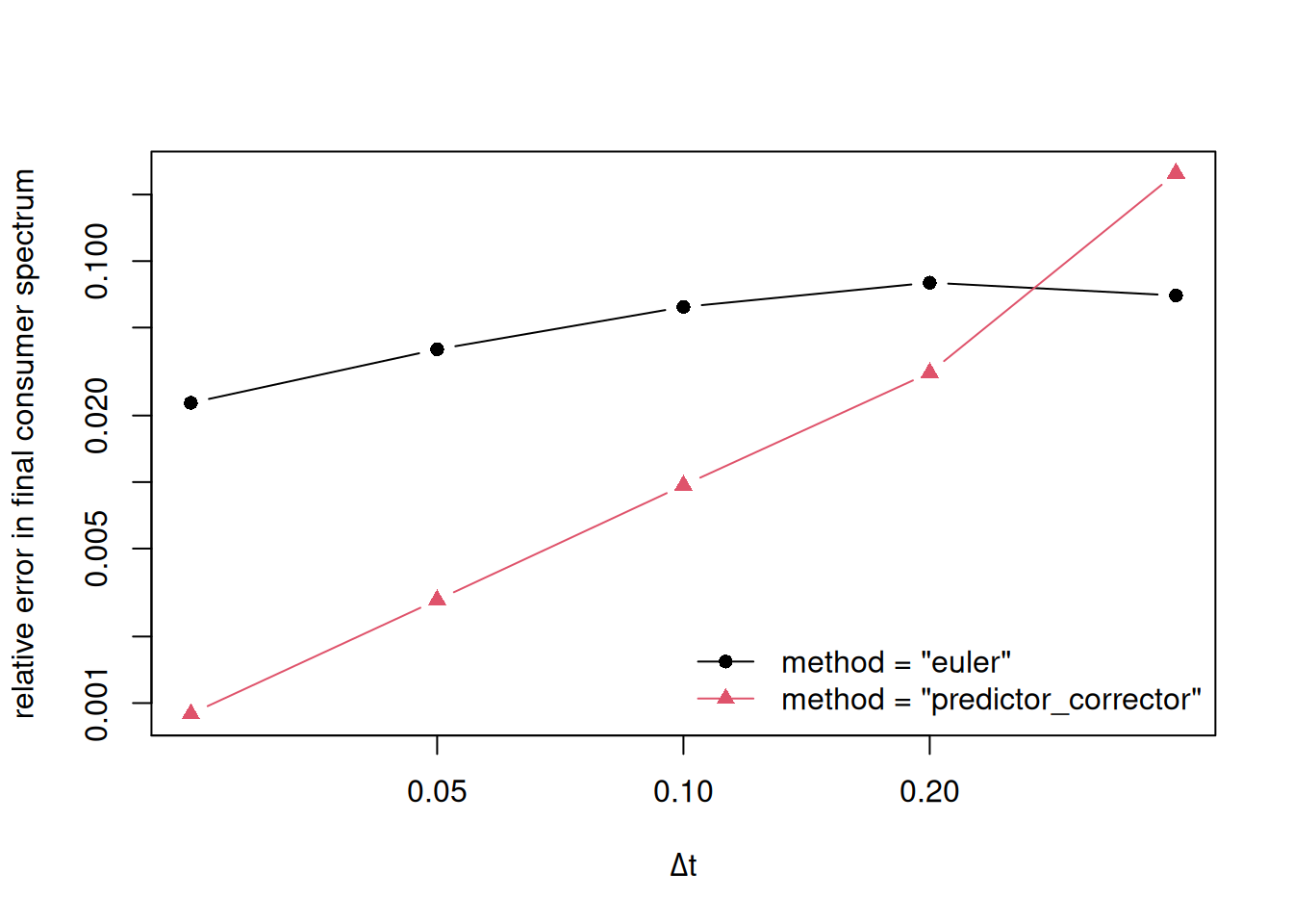
This vignette compares the first-order consumer density update, selected with method = "euler", with the two second-order updates selected with method = "predictor_corrector" and method = "tr_bdf2", on the North Sea example model NS_params.

The comparison is intentionally modest. It is meant as a reproducible smoke test for speed and time-step sensitivity, not as a comprehensive benchmark.

We compare final consumer spectra against a smaller-time-step reference solution from the TR-BDF2 method. Because all methods use the same spatial discretisation, this test is only about the time discretisation error on the fixed NS_params weight grid.

Code

t_max <- 8
dt_values <- c(1.6, 0.8,0.4, 0.2, 0.1, 0.05, 0.025)
reference_dt <- 0.4 / 2^6

params <- NS_params
initial_effort(params) <- 4

relative_l2_error <- function(x, reference) {
    x_final <- finalN(x)
    reference_final <- finalN(reference)
    sqrt(sum((x_final - reference_final)^2)) / sqrt(sum(reference_final^2))
}

reference <- project(
    params,
    dt = reference_dt,
    t_max = t_max,
    method = "tr_bdf2"
)

ℹ No `a` column so using a = 0.01 in w = a l^b, with w in g and l in cm.
ℹ No `b` column so using the isometric default b = 3 in w = a l^b.

Code

accuracy <- do.call(rbind, lapply(dt_values, function(dt) {
    euler <- project(params, dt = dt, t_max = t_max, t_save = t_max,
                     method = "euler")
    pc <- project(params, dt = dt, t_max = t_max, t_save = t_max,
                  method = "predictor_corrector")
    trbdf2 <- project(params, dt = dt, t_max = t_max, t_save = t_max,
                      method = "tr_bdf2")

    data.frame(
        dt = dt,
        euler_error = relative_l2_error(euler, reference),
        predictor_corrector_error = relative_l2_error(pc, reference),
        tr_bdf2_error = relative_l2_error(trbdf2, reference)
    )
}))

ℹ No `a` column so using a = 0.01 in w = a l^b, with w in g and l in cm.
ℹ No `b` column so using the isometric default b = 3 in w = a l^b.
ℹ No `a` column so using a = 0.01 in w = a l^b, with w in g and l in cm.
ℹ No `b` column so using the isometric default b = 3 in w = a l^b.
ℹ No `a` column so using a = 0.01 in w = a l^b, with w in g and l in cm.
ℹ No `b` column so using the isometric default b = 3 in w = a l^b.
ℹ No `a` column so using a = 0.01 in w = a l^b, with w in g and l in cm.
ℹ No `b` column so using the isometric default b = 3 in w = a l^b.
ℹ No `a` column so using a = 0.01 in w = a l^b, with w in g and l in cm.
ℹ No `b` column so using the isometric default b = 3 in w = a l^b.
ℹ No `a` column so using a = 0.01 in w = a l^b, with w in g and l in cm.
ℹ No `b` column so using the isometric default b = 3 in w = a l^b.
ℹ No `a` column so using a = 0.01 in w = a l^b, with w in g and l in cm.
ℹ No `b` column so using the isometric default b = 3 in w = a l^b.
ℹ No `a` column so using a = 0.01 in w = a l^b, with w in g and l in cm.
ℹ No `b` column so using the isometric default b = 3 in w = a l^b.
ℹ No `a` column so using a = 0.01 in w = a l^b, with w in g and l in cm.
ℹ No `b` column so using the isometric default b = 3 in w = a l^b.
ℹ No `a` column so using a = 0.01 in w = a l^b, with w in g and l in cm.
ℹ No `b` column so using the isometric default b = 3 in w = a l^b.
ℹ No `a` column so using a = 0.01 in w = a l^b, with w in g and l in cm.
ℹ No `b` column so using the isometric default b = 3 in w = a l^b.
ℹ No `a` column so using a = 0.01 in w = a l^b, with w in g and l in cm.
ℹ No `b` column so using the isometric default b = 3 in w = a l^b.
ℹ No `a` column so using a = 0.01 in w = a l^b, with w in g and l in cm.
ℹ No `b` column so using the isometric default b = 3 in w = a l^b.
ℹ No `a` column so using a = 0.01 in w = a l^b, with w in g and l in cm.
ℹ No `b` column so using the isometric default b = 3 in w = a l^b.
ℹ No `a` column so using a = 0.01 in w = a l^b, with w in g and l in cm.
ℹ No `b` column so using the isometric default b = 3 in w = a l^b.
ℹ No `a` column so using a = 0.01 in w = a l^b, with w in g and l in cm.
ℹ No `b` column so using the isometric default b = 3 in w = a l^b.
ℹ No `a` column so using a = 0.01 in w = a l^b, with w in g and l in cm.
ℹ No `b` column so using the isometric default b = 3 in w = a l^b.
ℹ No `a` column so using a = 0.01 in w = a l^b, with w in g and l in cm.
ℹ No `b` column so using the isometric default b = 3 in w = a l^b.
ℹ No `a` column so using a = 0.01 in w = a l^b, with w in g and l in cm.
ℹ No `b` column so using the isometric default b = 3 in w = a l^b.
ℹ No `a` column so using a = 0.01 in w = a l^b, with w in g and l in cm.
ℹ No `b` column so using the isometric default b = 3 in w = a l^b.
ℹ No `a` column so using a = 0.01 in w = a l^b, with w in g and l in cm.
ℹ No `b` column so using the isometric default b = 3 in w = a l^b.

Code

accuracy

     dt euler_error predictor_corrector_error tr_bdf2_error
1 1.600  0.31596647              3.4780282823  0.1485219020
2 0.800  0.15030919              1.5930749272  0.2161710472
3 0.400  0.06998422              0.2491341164  0.0858144631
4 0.200  0.07996242              0.0305651825  0.0305334237
5 0.100  0.06213206              0.0089017443  0.0091873340
6 0.050  0.03998051              0.0023680430  0.0024242194
7 0.025  0.02294875              0.0005722933  0.0005797011

Code

plot(
    euler_error ~ dt,
    data = accuracy,
    log = "xy",
    type = "b",
    pch = 16,
    xlab = expression(Delta * t),
    ylab = "relative error in final consumer spectrum",
    ylim = range(accuracy$euler_error, accuracy$predictor_corrector_error,
                 accuracy$tr_bdf2_error)
)
lines(
    predictor_corrector_error ~ dt,
    data = accuracy,
    type = "b",
    pch = 17,
    col = 2
)
lines(
    tr_bdf2_error ~ dt,
    data = accuracy,
    type = "b",
    pch = 15,
    col = 4
)
legend(
    "bottomright",
    legend = c('method = "euler"', 'method = "predictor_corrector"',
               'method = "tr_bdf2"'),
    pch = c(16, 17, 15),
    col = c(1, 2, 4),
    lty = 1,
    bty = "n"
)

Speed

The second-order methods do roughly twice the work per time step. The predictor-corrector method performs one predictor solve and then recalculates the rates before doing the corrector solve. TR-BDF2 performs the same predictor solve and rate recalculation, and then two stage solves against the shared operator, so it is marginally more expensive than the predictor-corrector method per step.

The resource update

Under the second-order methods the resource is also advanced to second order. The resource mortality \(\mu_R\) depends on the consumer densities, so evaluating it only at the start of the step would make the resource update first order and cap the overall accuracy. Instead, the predictor step is used to form the same midpoint rates \(r^{t+1/2}\) that drive the consumer corrector, and the resource is then advanced with the midpoint resource mortality \[ \mu_R^{t+1/2} = \tfrac{1}{2}\left(\mu_R^t + \hat\mu_R^{t+1}\right). \tag{55}\] At a steady state \(r^t = \hat r^{t+1} = r^{t+1/2}\), so the resource corrector reproduces the predictor and the steady state is unchanged. With the default semi-chemostat resource dynamics, which already use the analytic solution for fixed mortality, the remaining resource error is small, but the midpoint mortality removes the first-order time-stepping component. The euler method keeps the first-order resource update.

Interpretation

On short runs the second-order methods may not always show a clean second-order convergence slope because the comparison is affected by the fixed spatial grid, nonlinear rate feedbacks and ordinary timing noise. TR-BDF2 typically shows the cleanest slope of the three because, being L-stable, it does not ring at the larger time steps.

Because the predictor-corrector method is more expensive per time step, the relevant comparison is between the Euler method at a given dt and the predictor-corrector method at twice the dt so that both have similar run times.

Numerical Diffusion for the Predictor-Corrector Method

The predictor-corrector method uses the same upwind approximation in size as the first-order method, so it still has numerical diffusion. However, the Crank-Nicolson corrector changes the time-stepping contribution to that diffusion.

To see this, again consider the advection-only problem with constant growth rate \(g\) on a locally uniform grid with spacing \(\Delta w\): \[ \frac{\partial N}{\partial t} + g\frac{\partial N}{\partial w} = 0. \tag{56}\] With fixed rates, the corrector step reduces to the Crank-Nicolson upwind scheme \[ \frac{N_j^{t+1} - N_j^t}{\Delta t} + \frac{g}{2} \left[ \frac{N_j^{t+1} - N_{j-1}^{t+1}}{\Delta w} + \frac{N_j^t - N_{j-1}^t}{\Delta w} \right] = 0. \tag{57}\]

Expand this equation about the midpoint \((w_j, t + \Delta t / 2)\). The centred time difference gives \[ \frac{N_j^{t+1} - N_j^t}{\Delta t} = \frac{\partial N}{\partial t} + O(\Delta t^2). \tag{58}\] The average of the two upwind spatial differences gives \[ \frac{1}{2} \left[ \frac{N_j^{t+1} - N_{j-1}^{t+1}}{\Delta w} + \frac{N_j^t - N_{j-1}^t}{\Delta w} \right] = \frac{\partial N}{\partial w} - \frac{\Delta w}{2}\frac{\partial^2 N}{\partial w^2} + O(\Delta w^2) + O(\Delta t^2). \tag{59}\] Substituting these expansions into the scheme gives the modified equation \[ \frac{\partial N}{\partial t} + g\frac{\partial N}{\partial w} = \frac{g\Delta w}{2}\frac{\partial^2 N}{\partial w^2} + O(\Delta w^2) + O(\Delta t^2). \tag{60}\] Thus the numerical diffusivity in the usual advection-diffusion form is \[ D_{num}^{PC} = \frac{g\Delta w}{2}. \tag{61}\] In the mizer notation, where the diffusion term is written with a factor \(1/2\) inside the flux, this corresponds to the effective diffusion parameter \[ d_{num}^{PC}(w) \approx g(w)\Delta w. \tag{62}\] On the logarithmic grid this becomes \[ d_{num}^{PC}(w) \approx g(w)w\log\beta. \tag{63}\]

Compared with the first-order semi-implicit scheme, \[ d_{num}^{Euler}(w) \approx g(w)\Delta w + g(w)^2\Delta t, \tag{64}\] the predictor-corrector method removes the leading artificial diffusion proportional to \(\Delta t\). The remaining numerical diffusion is the spatial upwind diffusion, proportional to \(\Delta w\) or equivalently to \(\log\beta\) on the logarithmic grid. This is why decreasing \(\Delta t\) eventually stops improving the error much: once the time-stepping error is small, the spatial upwind error and other fixed discretisation errors dominate.

Reducing the Spatial Error: a Higher-Order Reconstruction

In the scheme above only one ingredient is first order: the upwind reconstruction of the boundary density in the advective flux (Equation 9). Using the bin-below average \(N_{j-1}\) as the density at the boundary \(w_j\) introduces the numerical diffusion \(d_{num}\approx g(w)\,w\log\beta\) derived earlier, and on a coarse logarithmic grid (a few hundred bins over many decades) it is not small. It is the one spatial error the second-order time methods cannot remove. The flux entry of the second_order_w slot replaces the upwind reconstruction by a higher-order one. Because the choice changes the discrete steady state it lives in the params object rather than being a project() argument.

The reconstruction

The boundary \(w_j\) is the midpoint, on the logarithmic axis, of the two bin centres \(w_{j-1}^c\) and \(w_j^c\), so a second-order estimate of the density there is the average of the two bin averages. We write the general reconstruction with a weight \(\chi_j\), \[ N(w_j) \approx N_{j-1} + \tfrac12\,\chi_j\,(N_j - N_{j-1}), \tag{65}\] which is pure upwind (\(N_{j-1}\)) when \(\chi_j = 0\) and the centred value \(\tfrac12(N_{j-1}+N_j)\) when \(\chi_j = 1\). The advective flux becomes \[ J_j^{adv} = g_j\bigl[N_{j-1} + \tfrac12\,\chi_j(N_j - N_{j-1})\bigr]. \tag{66}\] With \(\chi_j = 1\) the upwind numerical diffusion is gone and the advective flux is second order. The remaining requirement for a fully second-order model is that the bin-average rates — the diffusion coefficient \(d_j\) in the diffusive flux (Equation 10) and the mortality \(\mu_j\) in the sink (Equation 14) — actually be bin-averaged rather than point-sampled. That is the job of the bin_average entry of the slot, which gates exactly that point-versus-bin-average choice for \(d\) and \(\mu\) alike.

Choosing the weight: van Leer or centred

With \(\chi\equiv1\) the reconstruction is the pure centred one, which is genuinely second order everywhere, including at smooth extrema, but is not monotonicity-preserving: it can produce small over/undershoots, and at a steady state with no physical diffusion it admits an undamped odd-even mode. With the van Leer weight \[ \chi_j=\chi(r_j),\qquad \chi(r)=\frac{r+|r|}{1+|r|},\qquad r_j=\frac{N_{j-1}-N_{j-2}}{N_j-N_{j-1}}, \tag{67}\] the scheme is total-variation diminishing (TVD): \(\chi\to1\) where the solution is smooth, and \(\chi\to0\) (pure upwind) at extrema and at the non-smooth recruitment boundary. This keeps abundances non-negative and manufactures no new oscillations, at the price — a corollary of Godunov’s theorem — of dropping to first order at smooth extrema.

At the left boundary of the grid where \(N_{j-2}\) does not exist, the weight is handled as follows:

• At and below the first two faces above the recruitment boundary (\(j \le j_{min} + 2\)), the weight \(\chi_j\) is forced to 0. This keeps the advective flux leaving the recruitment boundary first-order upwind and avoids referencing the non-smooth recruitment boundary cell \(N_{j_{min}}\) (and the inactive region below it) when calculating the smoothness ratio, preventing ragged or oscillating solutions near the boundary.

The two types are selected with

second_order_w(params)$flux <- "van_leer" # TVD, the default for TRUE
second_order_w(params)$flux <- "centred"   # unlimited, true 2nd order

The default (TRUE) is van Leer, the safe choice for production runs; the centred reconstruction is most useful for smooth problems that carry some physical diffusion.

Implicit treatment with a frozen weight

The weight \(\chi_j\) is evaluated from the densities at the start of the step (for the second-order methods, from the midpoint field), so it is a fixed number during the solve. With \(\chi\) frozen, the flux Equation 66 is linear in the unknown densities \(N^{t+1}\) and still couples only \(N_{j-1},N_j,N_{j+1}\), so it folds directly into the same tridiagonal operator \(\tt{get\_transport\_coefs()}\) builds — only the advective coefficients gain the \(\chi\) terms. Keeping the high-order term implicit in this way is important: treating the extra (anti-diffusive) part explicitly on the right-hand side is only conditionally stable and breaks down for the lightly damped second-order time steppers, whereas the implicit form is stable for backward Euler and TR-BDF2 even with no physical diffusion.

Furthermore, because the van Leer weight \(\chi_j\) depends nonlinearly on the solution, naive time-stepping can fall into a limit cycle where \(\chi_j\) flip-flops between neighboring cells, preventing the solution from settling into a steady state. To break such limit cycles, mizer evaluates \(\chi_j\) with an exponential moving average (under-relaxation) across time steps: \(\chi_j^{(t)} = 0.5 \chi_j(N) + 0.5 \chi_j^{(t-1)}\). This relaxation only affects the transient approach and ensures the time-stepping iteration can smoothly reach the true fixed point.

The price is that the high-order term can make the off-diagonal coefficient \(C_j\) positive, so the operator is no longer an M-matrix and non-negativity is no longer guaranteed by construction. The van Leer reconstruction keeps any undershoot at the level of rounding, and the consumer update floors it to zero to preserve \(N\ge 0\); the unlimited centred reconstruction gives up this guarantee in exchange for the extra order.

Because the reconstruction weight is frozen at the beginning (or midpoint) of the step, the flux limiter is only conditionally total-variation diminishing (TVD). In simulations with highly dynamic, sharp features (such as pulsed reproduction starting from a zero initial abundance), the time step \(\Delta t\) must satisfy the Courant-Friedrichs-Lewy (CFL) condition, which requires that the log-size Courant number \[ C = \frac{g(w) \Delta t}{w \log\beta} \] be at most \(1\) across the grid. If the Courant number exceeds 1, the lagged limiter can no longer guarantee the TVD property, resulting in spurious oscillations (wiggles) and negative densities (which the update floors to zero, leading to a ragged/zero-interleaved distribution). To avoid wiggles in such cases, users should either reduce dt so that \(C \le 1\), or use the first-order upwind scheme (by setting second_order_w(params) <- FALSE and using the L-stable method = "tr_bdf2") which remains positive and monotonic for any dt.

Steady state and reproduction

Because the reconstruction lives entirely in the coefficients \(A,B,C\), the steady-state machinery stays consistent automatically: getRequiredRDD() reads the same boundary coefficients and get_steady_state_n() solves the same system. The exponential moving average under-relaxation in the van Leer weight \(\chi\) allows both the single-species steady state solver and the full multispecies solver = "project" time-stepping iteration to converge to the true discrete fixed point without falling into a limit cycle. Both getRequiredRDD() and steadySingleSpecies() read the same second_order_w slot, so a model is automatically set up at the steady state of exactly the scheme that project() will use, and that state is preserved to machine precision by all three time-stepping methods.

The direct solver reads its set of unknowns from where the supplied abundances are non-zero, rather than from \(w_{max}\). This keeps it robust when \(w_{max}\) is set far above the largest fish (a common choice, so that the grid need not change when a parameter update produces larger fish): the structurally-zero classes below such a \(w_{max}\) are simply excluded. The growth rate alone could not be used to find the support, because the main reason fish grow past \(w_{repro\_max}\) is diffusion, whose rate only grows with \(w\) and never vanishes; the abundance is the only reliable indicator of where the (possibly diffusion-fed) tail has died away. With the van Leer limiter the residual is only Lipschitz, so the Newton iteration converges to a fixed point of the dynamics but not to machine precision; the unlimited centred reconstruction — which admits an undamped odd-even mode at a steady state with no physical diffusion — gives an ill-conditioned steady-state Jacobian for which the direct solver is not expected to converge.

Steady-State Solution

When solving the steady-state ODE instead of the time-dependent PDE, we are looking for a state where the population densities do not change over time, meaning \(N_j^{t+1} = N_j^t = N_j^*\).

Substituting this into our discretised linear system: \[ A_j N_{j-1}^* + B_j N_j^* + C_j N_{j+1}^* = S_j \tag{68}\] Recall that for \(j > j_{min}\), \(S_j = N_j^t\). The equation simplifies to: \[ A_j N_{j-1}^* + (B_j - 1) N_j^* + C_j N_{j+1}^* = 0 \tag{69}\]

To find the steady-state population densities \(N^*\), we formulate a new time-independent tridiagonal system: \[ \tilde{A}_j N_{j-1}^* + \tilde{B}_j N_j^* + \tilde{C}_j N_{j+1}^* = \tilde{S}_j \tag{70}\] To eliminate the explicit dependence on the time step \(\Delta t\), we can divide the equation by \(\Delta t\). The modified coefficients \(\tilde{A}, \tilde{B}, \tilde{C}\) defining the new tri-diagonal system are: \[ \begin{aligned} \tilde{A}_j &= \frac{A_j}{\Delta t} = -\frac{1}{\Delta w_j} \left( g_j + \frac{1}{2} \frac{d_{j-1}}{\Delta w_{j-1}^c} \right) \\ \tilde{C}_j &= \frac{C_j}{\Delta t} = -\frac{1}{\Delta w_j} \left( \frac{1}{2} \frac{d_{j+1}}{\Delta w_j^c} \right) \\ \tilde{B}_j &= \frac{B_j - 1}{\Delta t} = \mu_j + \frac{1}{\Delta w_j} \left( g_{j+1} + \frac{1}{2} \frac{d_j}{\Delta w_j^c} + \frac{1}{2} \frac{d_j}{\Delta w_{j-1}^c} \right) \end{aligned} \tag{71}\] Notice that \(\tilde{A}_j\) and \(\tilde{C}_j\) are exactly the expressions for \(A_j\) and \(C_j\) evaluated at \(\Delta t = 1\). Similarly, \(\tilde{B}_j\) is exactly the expression for \(B_j - 1\) evaluated at \(\Delta t = 1\).

Boundary conditions for the steady state:

For the smallest size (\(j=j_{min}\)), the original equation had a source term due to recruitment: \[ S_{j_{min}} = N_{j_{min}}^t + \frac{\Delta t}{\Delta w_{j_{min}}} R_{dd} \tag{72}\] Following the same logic of setting \(N^{t+1} = N^t = N^*\) and dividing by \(\Delta t\), the right-hand side vector \(\tilde{S}_j\) for the steady-state system becomes purely the recruitment flux term. If we again observe the original term \(\frac{\Delta t}{\Delta w_{j_{min}}} R_{dd}\) when evaluated at \(\Delta t = 1\), we get our new source vector: \[ \tilde{S}_{j_{min}} = \frac{R_{dd}}{\Delta w_{j_{min}}} \tag{73}\] For all other \(j > j_{min}\), \(\tilde{S}_j = 0\).

The boundary condition modifications at the edges of the grid remain the same conceptually: \(\tilde{A}_{j_{min}} = 0\), the upward diffusion term is omitted from \(\tilde{B}_{j_{min}}\), and \(\tilde{C}_{j_{max}} = 0\), where \(j_{max}\) is the support top of the previous section (the first class above \(w_{max}\)). The density is held at zero for any \(j < j_{min}\) or \(j > j_{max}\).

In code, this means that the steady-state coefficients for the matrix multiplication (\(\tilde{A}, \tilde{B}, \tilde{C}\)) and the constant vector (\(\tilde{S}\)) can be calculated by calling the standard coefficient function but simply setting \(\Delta t = 1\), and dropping the \(+1\) and \(+N_j^t\) from the resulting \(B\) and \(S\) variables respectively.

With these modified matrices, the steady-state densities can be calculated directly by solving the linear system avoiding the need to iterate step by step over time.

Steady-State Solution for the Predictor-Corrector Method

The predictor-corrector method changes the time stepping, but it does not change the steady state that is obtained when the rates are evaluated at that steady state. To see this, write the Crank-Nicolson corrector with fixed midpoint rates as \[ \frac{N^{t+1} - N^t}{\Delta t} = \frac{1}{2}\left(L N^t + L N^{t+1}\right) + q, \tag{74}\] where \(L\) is the spatial transport-and-mortality operator built from the midpoint rates and \(q\) is the recruitment source at the lower boundary. At a steady state, \(N^{t+1} = N^t = N^*\), so this becomes simply \[ 0 = L N^* + q. \tag{75}\]

Thus the predictor-corrector method has the same fixed-point equation as the first-order method. The predictor step also becomes irrelevant at the fixed point: if \(N^t = N^*\), then the predicted \(\hat{N}^{t+1}\) is also \(N^*\) up to the residual of the steady-state equation, so \[ r^t = \hat{r}^{t+1} = r^{t+1/2}, \qquad R_{dd}^t = \hat{R}_{dd}^{t+1} = R_{dd}^{t+1/2}. \tag{76}\] The rates used in the steady-state calculation are therefore just the rates evaluated at \(N^*\). The predictor-corrector method affects the transient path to the steady state, not the steady state itself.

Direct Steady-State Solver (solver = "newton")

With solver = "newton", tuneSteadyState() and findSteadyState() find the steady state by directly solving the discretised algebraic equation \(F(N) = 0\) (derived in the sections above) using a Newton-type root finder. This allows them to converge to the steady state even when the state is dynamically unstable.

To make the nonlinear algebraic system well-behaved for the root finder, the solver employs several numerical strategies:

1. Log-space solve: The consumer densities are solved for in logarithmic space (\(x = \log N\)). This enforces strict positivity of the densities during the iteration and natively conditions the Jacobian by turning absolute density perturbations—which span dozens of orders of magnitude—into well-scaled \(O(1)\) relative (multiplicative) perturbations. The residual of the equation is correspondingly scaled by \(1/N\), turning it into a per-capita rate of change that is also \(O(1)\) across all size classes.

2. Active support and structural zeros: The solver defines the “active” size classes for each species as running from the egg size up to the overall grid truncation limit, regardless of whether they initially carry non-zero density. Because the logarithm of zero is \(-\infty\), the solver applies a smooth, continuous penalty floor to the log-abundances. This automatically bounds the unknowns, gracefully handling structurally zero-density classes and preventing singular Jacobians. After convergence, densities that remain trapped at or near this penalty floor are explicitly set to exactly zero. This allows the solver to automatically discover the true support (the highest non-zero size class) of the steady state.

3. Interaction with high-order spatial schemes: The solver strictly respects the spatial transport scheme configured in the parameters (e.g., via second_order_w()). The nonlinear flux limiter weight is recalculated at every residual evaluation, ensuring the returned steady state is an exact fixed point of the chosen dynamics. However, because the TVD “van Leer” flux limiter is only Lipschitz-continuous (its derivative is discontinuous where the smoothness indicator equals 1), the Newton iteration converges to the fixed point but typically not to machine precision. Conversely, the unlimited “centred” reconstruction is perfectly smooth, but at a steady state with no physical diffusion it admits an undamped odd-even mode, leading to a structurally ill-conditioned Jacobian for which the Newton solver is unlikely to converge.

Linear Stability Analysis

Once a steady state \(N^*\) has been found, mizer can evaluate its dynamic stability by linearising the discrete-time map around \(N^*\). The time step acts as a map \(N^{t+1} = G(N^t)\), and the stability of the steady state is governed by the eigenvalues of the absolute Jacobian matrix \(L\): \[ L_{ij} = \frac{\partial G_i}{\partial N_j}(N^*) \tag{77}\]

Multiplicative Finite Differences

Because abundances in a mizer model span dozens of orders of magnitude, evaluating the Jacobian \(L\) numerically using a constant absolute perturbation size (e.g., \(N_j^* + \epsilon\) with \(\epsilon = 10^{-4}\)) is poorly scaled. The perturbation would be lost in rounding error for larvae, and catastrophically huge for large fish.

Instead, the getStability() function approximates the derivative using a multiplicative (relative) finite-difference step. It perturbs the abundance \(N_j^*\) by an amount \(\Delta N_j\) proportional to the steady-state abundance: \[ \Delta N_j = h \cdot \max(N_j^*, \text{machine eps}) \tag{78}\] where \(h\) is the relative step size (default \(10^{-4}\)). The function then evaluates the system’s response: \[ L_{ij} \approx \frac{G_i(N^* + \Delta N_j) - G_i(N^* - \Delta N_j)}{2 \Delta N_j} \tag{79}\] This ensures the numerical precision is maintained across all size classes. A tiny additive floor (the machine epsilon) is kept to allow the solver to gently “poke” classes where the steady-state abundance is exactly zero (like extinct species or the truncated tail above \(w_{max}\)), capturing their stability against small invasions.

Equivalence to Log-Space Analysis

It might seem conceptually more natural to analyse stability entirely in log-space, by perturbing the relative abundances \(x_j(t) = (N_j(t) - N_j^*) / N_j^*\) and computing the relative Jacobian \(K\): \[ K_{ij} = \frac{\partial \log G_i}{\partial \log N_j} \tag{80}\]

Applying the chain rule, this log-space Jacobian relates to the absolute Jacobian via: \[ K_{ij} = \frac{\partial \log G_i}{\partial G_i} \frac{\partial G_i}{\partial N_j} \frac{\partial N_j}{\partial \log N_j} = \frac{1}{N_i^*} L_{ij} N_j^* \tag{81}\] In matrix notation, this is a similarity transform: \(K = D^{-1} L D\), where \(D\) is a diagonal matrix containing the steady-state abundances \(N^*\).

A fundamental theorem of linear algebra states that similar matrices have exactly the same eigenvalues. Because stability is determined entirely by whether any eigenvalue’s modulus exceeds 1, \(L\) and \(K\) yield mathematically identical stability conclusions.

Numerically, however, explicitly computing the relative Jacobian \(K\) requires dividing the elements of \(L\) by the steady-state abundances \(N_i^*\). For structurally zero size classes, this division by zero causes floating-point overflow (Inf or NaN), breaking standard eigenvalue solvers. Therefore, getStability() numerically computes the well-conditioned absolute Jacobian \(L\) (using the multiplicative-scale finite difference) and relies on the similarity equivalence to guarantee the correct result.