Overview
The mizer package implements multi-species dynamic Size-spectrum models in R. It has been designed for modelling aquatic ecosystems.
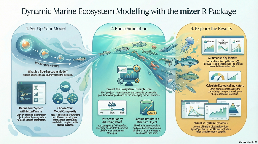
Using mizer is relatively simple. There are four main stages, each described in more detail in sections below.
Once you have seen these stages individually, the worked example near the end of this page puts them together into a complete, self-contained study of a real ecosystem — building, calibrating and projecting a Celtic Sea model.
If you run into any difficulties or have any questions or suggestions, let us know about it by posting about it on our issue tracker. You can also twitter to @mizer_model. We love to hear from you.
A good way to get into mizer is to follow the online mizer course. This course has three parts, each consisting of several tutorials with example code and exercises:
Part 1: Understand
You will gain an understanding of size spectra and their dynamics by exploring simple example systems hands-on with mizer.Part 2: Build
You will build your own multi-species mizer model for the Celtic sea, following our example. You can also create a model for your own area of interest.Part 3: Use
You will explore the effects of changes in fishing and changes in resource dynamics on the fish community and the fisheries yield. You will run your own model scenarios.
Click on this preview to open a mizer cheat sheet. 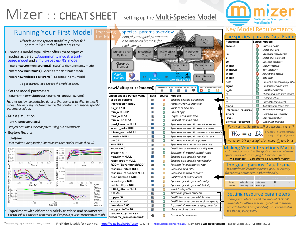
For quick reference while working we also provide four topic-based cheat sheets:
There is a series of YouTube videos by Richard Southwell about mizer which are however no longer entirely up-to-date.
Installing mizer
If you already have R installed on your computer, then installation of the mizer package is very simple (assuming you have an active internet connection). Just start an R session and then type:
install.packages("mizer")After installing mizer, to actually use it, you need to load the
package using the library() function. Note that whilst you
only need to install the package once, it will need to be loaded every
time you start a new R session.
Mizer is compatible with R versions 3.5 and later. You can install R on your computer by following the instructions at https://cran.r-project.org/ for your particular platform.
Alternatively, if you can not or do not want to install R on your computer, you can also work with R and RStudio in your internet browser by creating yourself a free account at https://rstudio.cloud. There you can then install mizer as described above. Running mizer in the RStudio Cloud may be slightly slower than running it locally on your machine, but the speed is usually quite acceptable.
This guide assumes that you will be using RStudio to work with R. There is really no reason not to use RStudio and it makes a lot of things much easier. RStudio develops rapidly and adds useful features all the time and so it pays to upgrade to the latest version frequently. This guide was written with version 2023.12.1.
The source code for mizer is hosted on GitHub. If you are feeling brave and wish to try out a development version of mizer you can install the package from here using the R package devtools (which was used extensively in putting together mizer). If you have not yet installed devtools, do
install.packages("devtools")Then you can install the latest version from GitHub using
devtools::install_github("sizespectrum/mizer")devtools::install_github() function you can
also install code from forked mizer repositories or from other branches
on the official repository.
Setting the model parameters
With mizer it is possible to implement many different types of size-spectrum models using the same basic tools and methods.
Setting the model parameters is done by creating an object of
class ? MizerParams. This includes model parameters such as
the life history parameters of each species, and the fishing gears. For
each type of sizespectrum model there is a function for creating a new
MizerParams object, newSingleSpeciesParams(),
newCommunityParams(), newTraitParams() and
newMultispeciesParams().
These functions make reasonable default choices for many of the model parameters that you do not want to specify explicitly. For example to set up a simple model (described more in the Community Model section) you can even let mizer choose all the parameters for you.
params <- newCommunityParams()For a more complicated multi-species model you need to provide a data frame with some species parameters. An example of a North Sea model is included with the package. Here we also use a species interaction matrix for the North Sea species.
params <- newMultispeciesParams(NS_species_params, NS_interaction)When you run this yourself, the function prints some notes explaining
that, because only a few species parameters were supplied, mizer has
calculated default values for many others (for example the maximum
intake rate h and the search volume gamma)
using size-based theory. These notes are informational, not errors: they
simply flag the parameters you may want to refine later once you
calibrate the model to data. We have suppressed them here to keep the
output short. Calibrating such a model to observed biomasses and yields
is demonstrated in the worked
example below.
Running a simulation
This is done by calling the project() function (as in
“project forward in time”) with the model parameters.
sim <- project(params, t_max = 10, effort = 1)This produces an object of class MizerSim which contains
the results of the simulation. In this example we chose to set some
parameters of the project() function to specify that we
want to project 10 years into the future, under the assumption of unit
fishing effort. You can see the help page for project() for
more details and it is described fully in the
section on running a simulation.
Exploring the results
After a simulation has been run, the results can be examined using a
range of ?plotting_functions,
?summary_functions and ?indicator_functions.
The plot() function combines several of these plots into
one:
plot(sim)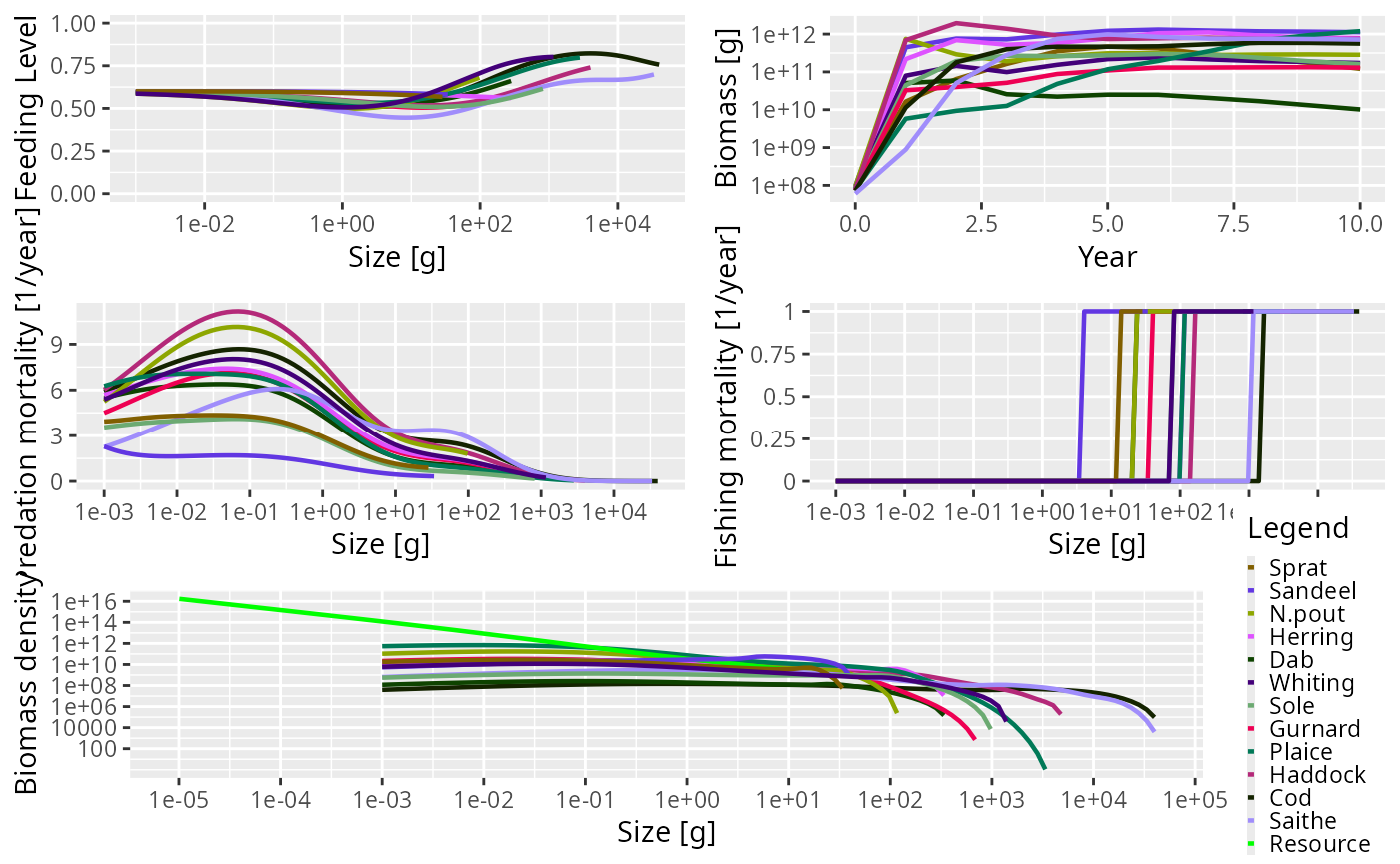
Just as an example: we might be interested in how the proportion of large fish varies over time. We can get the proportion of Herrings in terms of biomass that have a weight above 50g in each of the 10 years:
getProportionOfLargeFish(sim,
                         species = "Herring",
                         threshold_w = 50,
                         biomass_proportion = TRUE)
## 0 1 2 3 4 5 6 7
## 0.8241807 0.1858698 0.7586884 0.6780193 0.3325129 0.3036110 0.4717033 0.6379461
## 8 9 10
## 0.5976582 0.5539731 0.5763835We can then use the full power of R to work with these results.
The functionality provided by mizer to explore the simulation results is more fully described in the section on exploring the simulation results.
A worked example: the Celtic Sea
The four stages above introduced the mizer API one command at a time. This section puts them together into a single, self-contained study of a real ecosystem — the Celtic Sea — taking a model from raw species parameters all the way to a fishing-scenario result:
- Build a multi-species model from species parameters, an interaction matrix and fishing-gear definitions.
- Bring it to steady state so the size spectra are self-consistent.
- Calibrate it so that its steady state reproduces the observed biomasses and growth rates.
- Check it against an independent quantity — the observed fisheries yields.
- Set its resilience to fishing.
- Project a fishing scenario and interpret an indicator — here, the total sustainable yield as a function of fishing effort.
The model is the one built step-by-step, with much more explanation of every choice, in the Build part of the mizer course. It is based on the Celtic Sea model of Spence et al. (2021), with species parameters and observations drawn from FishBase and the ICES stock-assessment database. Here we concentrate on seeing the whole workflow run in one place.
Getting the data
The model needs three inputs: a species-parameter data frame, a species interaction matrix, and a table of fishing-gear parameters. We also load a set of observed commercial yields to check the model against later. These small files live in the course repository; the code below downloads them into your working directory the first time you run it.
base_url <- "https://github.com/gustavdelius/mizerCourse/raw/master/build/"
files <- c("celtic_species_params.rds", "celtic_gear_params.csv",
           "celtic_interaction.csv", "celtic_yields.rds")
for (f in files) {
    if (!file.exists(f)) download.file(paste0(base_url, f), destfile = f)
}

celtic_species_params <- readRDS("celtic_species_params.rds")
celtic_gear_params    <- read.csv("celtic_gear_params.csv")
celtic_interaction    <- as.matrix(read.csv("celtic_interaction.csv",
                                             row.names = 1))
The species-parameter data frame has one row per species. Besides the
required maximum size w_max it carries a few life-history
parameters and, crucially, the observed average biomass
of each species (biomass_observed, in grams per square
metre) that we will calibrate to. Some species have no observation and
are left as NA.
celtic_species_params[, c("species", "w_max", "biomass_observed")]## species w_max biomass_observed
## 1 Herring 307.31559 0.300000000
## 2 Sprat 35.84195 0.295749801
## 3 Cod 41561.32628 0.008179382
## 4 Haddock 6669.92227 0.067381049
## 5 Whiting 2611.42837 0.070079361
## 6 Blue whiting 599.82211 1.188248745
## 7 Norway Pout 319.77787 0.172520253
## 8 Poor Cod 711.87913 NA
## 9 European Hake 15506.13615 0.164362236
## 10 Monkfish 21478.67091 0.048720611
## 11 Horse Mackerel 518.58232 NA
## 12 Mackerel 1857.47965 NA
## 13 Common Dab 640.30873 NA
## 14 Plaice 3133.64249 0.022404698
## 15 Megrim 1556.92834 0.074079322
## 16 Sole 1979.31808 0.063519261
## 17 Boarfish 278.92128 NABuilding the model
newMultispeciesParams() turns these inputs into a
MizerParams object, filling in with size-based defaults
every parameter we have not supplied. We set the allometric exponents
n and p both to 3/4 and switch the commercial
gear on at unit effort.
cel <- newMultispeciesParams(
    species_params = celtic_species_params,
    gear_params    = celtic_gear_params,
    interaction    = celtic_interaction,
    n = 3/4, p = 3/4,
    initial_effort = 1
)
As before, mizer prints notes about the defaults it has chosen; we have suppressed them here to keep the output short.
Finding the steady state
A freshly built model has only a rough spectrum.
steady() runs the size-spectrum dynamics, holding
reproduction and the resource fixed, until the community settles onto a
steady state.
cel <- steady(cel)
plotSpectra(cel, power = 2)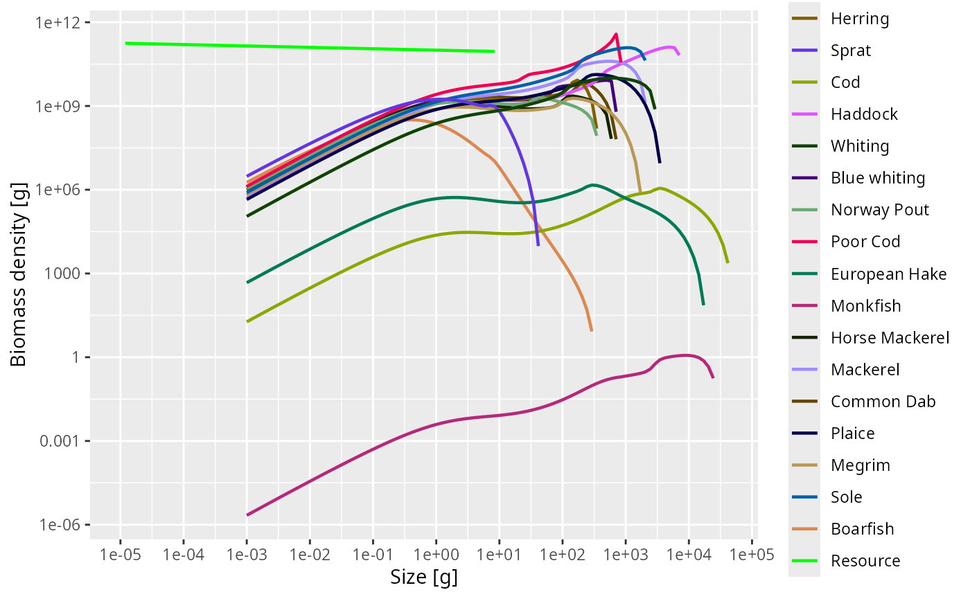
Each curve is now a smooth species spectrum, and together they line up along the background resource — the hallmark of a self-consistent size-spectrum model.
Calibrating to observed biomass
The steady state is self-consistent, but its species abundances are
still arbitrary. Calibration rescales them to match observation. We do
this in stages, re-running steady() after every
adjustment because each change pushes the community off its
steady state:
-
calibrateBiomass()sets the overall abundance scale (the resource levelkappa) so that the total community biomass matches the sum of the observed biomasses. -
matchBiomasses()then rescales each species individually to its ownbiomass_observed. -
matchGrowth()adjusts intake, search volume and metabolism so the fish reach maturity at the right age.
matchBiomasses() and matchGrowth() pull on
different parameters, so we alternate them, re-converging each time,
until both are satisfied.
cel <- calibrateBiomass(cel)
for (i in 1:4) {
    cel <- matchBiomasses(cel)
    cel <- matchGrowth(cel)
    cel <- steady(cel)
}
plotBiomassObservedVsModel() shows how well the
calibrated steady state reproduces the observations: points on the
diagonal are a perfect match.
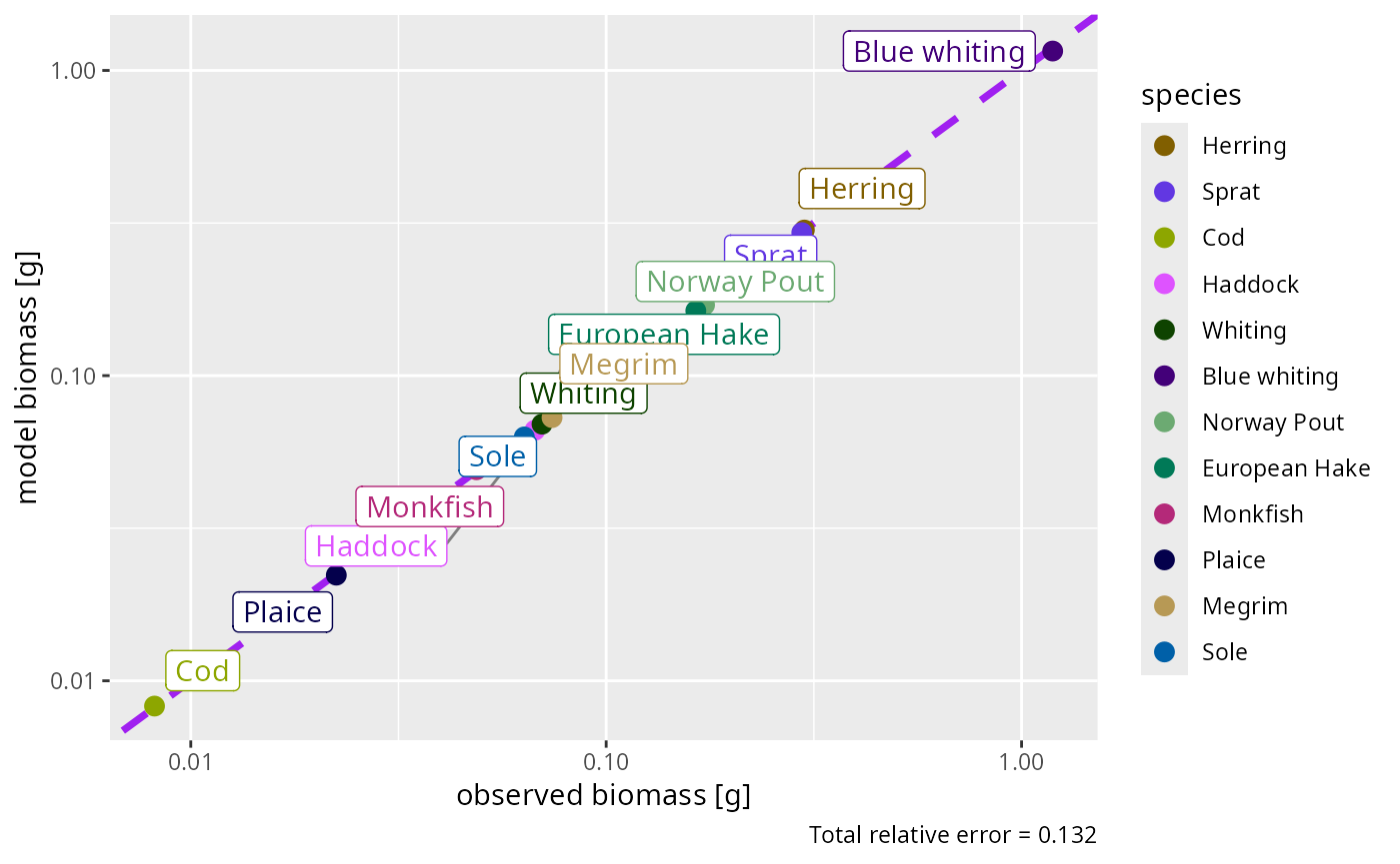
Most species sit close to the 1:1 line. A few remain off — the worst by nearly an order of magnitude — and these would need more iteration, or a look at their predation-kernel parameters, before you trusted the model for them. Diagnosing and fixing such residuals is exactly what the refinement tutorial of the course is about.
Checking against observed yield
Biomass was our calibration target. The fisheries yield is an independent quantity: we did not tune to it, so comparing modelled and observed yields is a genuine test of the model. We attach the observed yields and plot them against the model.
celtic_yields <- readRDS("celtic_yields.rds")
species_params(cel)$yield_observed <- as.numeric(celtic_yields)
plotYieldObservedVsModel(cel)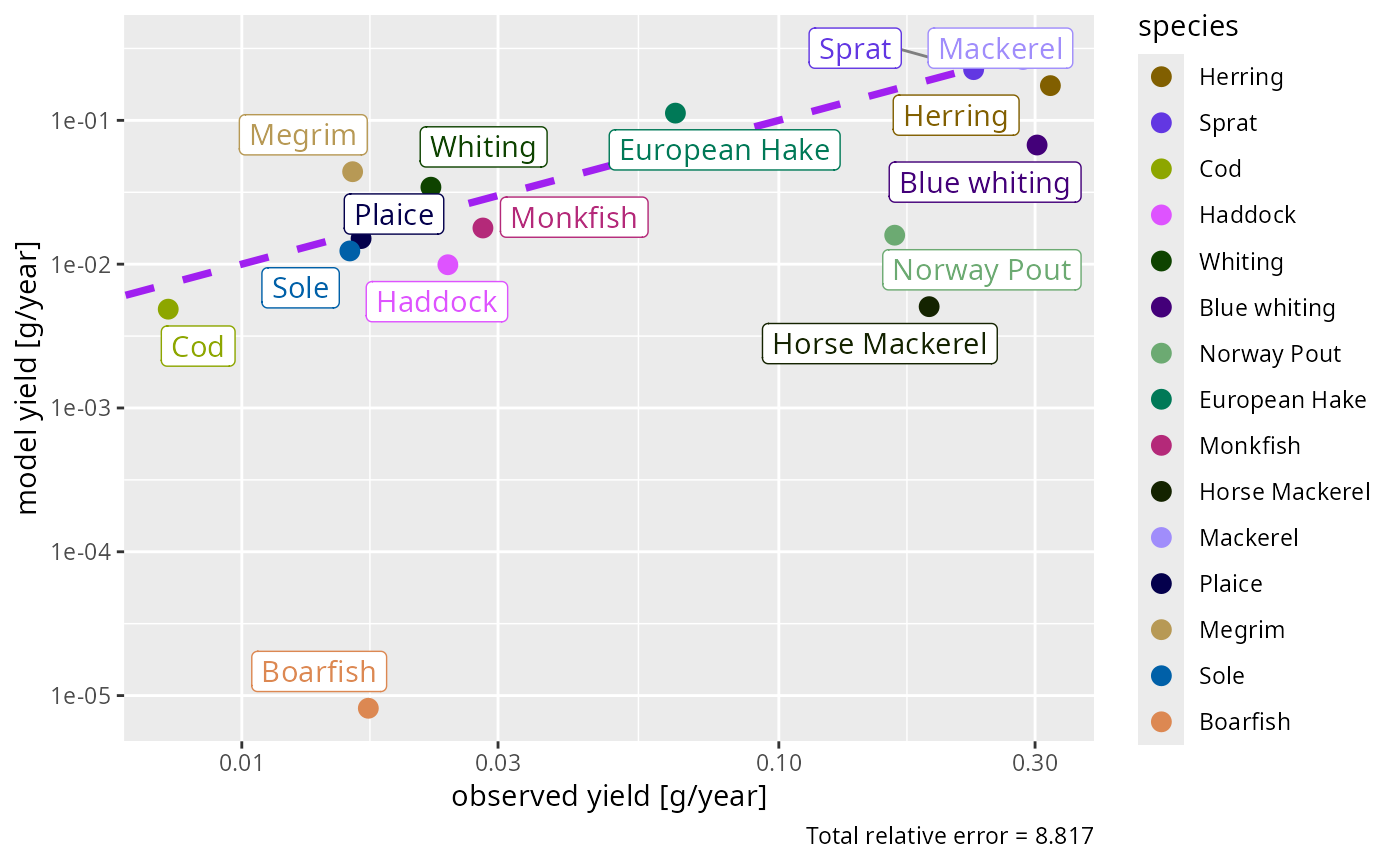
The modelled yields come out at the right overall level and mostly within a factor of a few of the observations — reassuring, given that yield was not a calibration target. Where a species’ yield is badly off, the usual culprit is its gear selectivity or catchability, which you would adjust next (see the landings tutorial).
Setting the resilience to fishing
Calibrating the steady state fixes where the community sits,
but not how sensitively it responds when we change fishing.
That sensitivity is governed by the strength of density dependence in
reproduction. setBevertonHolt() sets it through the
reproduction_level — the fraction of the maximum
recruitment that is realised at the steady state. A value of 0.5 gives
moderate density dependence, a common default in the absence of
stock-specific information.
cel <- setBevertonHolt(cel, reproduction_level = 0.5)This changes the reproduction parameters without moving the steady state, so the biomass and yield fits above are preserved.
Projecting a fishing scenario
We now have a calibrated, resilient model. Let us use it to ask a management question: is the fishery being fished at the effort that maximises the total sustainable yield?
We sweep fishing effort from zero to twice its current value. For each level we project to the new steady state and record the total community yield — the yield that could be taken indefinitely at that effort.
efforts <- c(0, 0.25, 0.5, 0.75, 1, 1.25, 1.5, 2)
sustainable_yield <- sapply(efforts, function(e) {
    p <- projectToSteady(cel, effort = e, t_max = 100,
                         return_sim = FALSE, progress_bar = FALSE)
    sum(getYield(p))
})

plot(efforts, sustainable_yield, type = "b", pch = 19,
     xlab = "Fishing effort (relative to current)",
     ylab = "Total sustainable yield (g/m²/year)")
abline(v = 1, lty = 2)
Interpreting the result
The curve is the community-level analogue of a single-stock yield curve. It rises, peaks, and then falls as heavier fishing starts to erode the stocks faster than they can rebuild. The dashed line marks the current effort.
The peak — the effort giving maximum sustainable yield for the community as a whole — lies a little below the current effort. In other words, this fishery is already working slightly harder than the level that would maximise its total long-term catch: pushing effort higher buys no extra yield and depletes the community, while easing off a little would increase the sustainable catch. That is a textbook signature of a lightly overfished community, recovered here purely from the model we calibrated to biomass and growth.
This is only the beginning of what the calibrated model can tell you.
From here you could look at individual species’ yield curves to find
each stock’s own \(F_\text{MSY}\)
(plotYieldVsF()), change the gear selectivity to protect
juveniles, or explore how the community size spectrum flattens under
fishing. The Use
part of the course develops several such scenarios.
Size-spectrum models
Size spectrum models have emerged as a conceptually simple way to model a large community of individuals which grow and change trophic level during life. There is now a growing literature describing different types of size spectrum models (e.g. Benoît and Rochet 2004; Andersen and Beyer 2006; Andersen et al. 2008; Law et al. 2009; Hartvig 2011; Hartvig et al. 2011). The models can be used to understand how marine communities are organised (Andersen and Beyer 2006; Andersen et al. 2009; Blanchard et al. 2009) and how they respond to fishing (Andersen and Rice 2010; Andersen and Pedersen 2010). This section introduces the central assumptions, concepts, processes, equations and parameters of size spectrum models.
Roughly speaking there are four versions of the size spectrum modelling framework of increasing complexity: The single-species model, the community model (Benoît and Rochet 2004; Maury et al. 2007; Blanchard et al. 2009; Law et al. 2009), the trait-based model (Andersen and Beyer 2006; Andersen and Pedersen 2010), and the multispecies model (Hartvig et al. 2011). The single-species, community and trait-based models can be considered as simplifications of the multispecies model. This section focuses on the multispecies model but is also applicable to the other types of models. Mizer is able to implement all types of model using similar commands.
Size spectrum models are a subset of physiologically structured models (Metz and Diekmann 1986; De Roos and Persson 2001) as growth (and thus maturation) is food dependent, and processes are formulated in terms of individual level processes. All parameters in the size spectrum models are related to individual weight which makes it possible to formulate the model with a small set of general parameters, which has prompted the label ``charmingly simple’’ to the model framework [Pope et al. (2006)}.
The model framework builds on the central assumption that an individual can be characterized by its weight \(w\) and its species number \(i\) only. The aim of the model is to calculate the size- and trait-spectrum \({\cal N}_i(w)\) which is the density of individuals such that \({\cal N}_i(w)dw\) is the number of individuals in the interval \([w:w+dw]\). Scaling from individual-level processes of growth and mortality to the size spectrum of each trait group is achieved by means of the McKendrick-von Foerster equation, which is simply a continuity equation that describes the flow of biomass up the size spectrum, \[\begin{equation} \frac{\partial N_i(w)}{\partial t} + \frac{\partial g_i(w) N_i(w)}{\partial w} = -\mu_i(w) N_i(w) \end{equation}\] where individual growth \(g_i(w)\) and mortality \(\mu_i(w)\) are coupled, because growth of one individual is due to predation on another, who consequently dies.
The continuity equation is supplemented by a boundary condition at the egg weight \(w_0\) where the flux of individuals (numbers per time) \(g_i(w_0) N_i(w_0)\) is determined by the reproduction of offspring by mature individuals in the population \(R_i\): \[\begin{equation} g_i(w_0)N_i(w_0) = R_i. \end{equation}\]
The rest of the formulation of the model rests on a number of ``standard’’ assumptions from ecology and fisheries science about how encounters between predators and prey leads to growth \(g_i(w)\) and reproduction \(R_i\) of the predators, and mortality of the prey \(\mu_i(w)\).
For a more detailed exposition of the model see the section The mizer size-spectrum model.
It is easiest to learn the basics of mizer through examples. We do this by looking at four set-ups of the framework, of increasing complexity. For each one there is an article that describes how to set up the model, run it in different scenarios, and explore the results. We recommend that you explore these in the following order:
Single-species model
The single-species model is a good starting point because it allows one to understand the main features of size-spectrum modelling without the complexities of multi-species interactions. The model describes a single species in a fixed background community. It allows exploration of how the shape of the species size spectrum is determined by the growth and death rates of individuals of that species. The article gives you a first glimpse of how to work with mizer, but in a simplified setting.
Community model
In the community model, individuals are only characterized by their size and are represented by a single group representing an across-species average. Community size spectrum models have been used to investigate how abundance size spectra emerge solely from the individual-level process of size-based predation and how fishing impacts metrics of community-level size spectra. Since few parameters are required it has been used for investigating large-scale community-level questions where detailed trait- and species-level parameterisations are not tractable.
Trait-based model
The trait-based model resolves a continuum of species with varying maximum sizes. The maximum size is considered to be the most important trait that characterizes a species’ life history. The continuum is represented by a discrete number of species spread evenly over the range of maximum sizes. The number of species is not important and does not affect the general dynamics of the model. Many of the parameters, such as the preferred predator-prey mass ratio, are the same for all species. Other model parameters are determined by the maximum size. For example, the weight at maturation of each species is a set fraction of the maximum size. In the trait-based model, species-level complexity is captured through different life histories, and both intra- and inter-specific size spectra emerge. This approach is powerful for examining the generic population and whole community level responses to both size and species selective fishing without the requirement for detailed species-specific parameters.
Multispecies model
In the multispecies model individual species are resolved in detail and each has distinct life history, feeding and reproduction parameters. More detailed information is required to parameterise the multispecies model but the approach can be used to address management strategies for a realistic community in a specific region or subset of interacting species.
Which model to use
All models predict abundance, biomass and yield as well as predation and mortality rates at size. They are useful for establishing baselines of abundance of unexploited communities, for understanding how fishing impacts aquatic communities and for testing indicators that are being developed to support an ecosystem approach to fisheries management.
Which model to use in a specific case depends on needs and on the amount of information available to calibrate the model. The multi-species model could be set up for most systems where calibration parameters can be estimated. This requires a lot of insight and data. If the parameters are just guesstimates the results of the multi-species model will be no more accurate than the results from the trait-based model. In such situations we therefore recommend the use of the trait-based model, even though it only provides general information about the maximum size distribution and not about specific species.
The community model is useful for large-scale community-level questions where only the average spectrum is needed. Care should be taken when the community model is used to infer the dynamical properties of marine ecosystems, since it is prone to unrealistically strong oscillations due to the lack of dampening effects provided by the life-history diversity in the trait-based and multi-species models.
The single-species model is mainly of pedagogical use and for comparison to other single-species fisheries models. But an important aim of size-spectrum modelling is to get away from single-species thinking.
Using AI coding agents with mizer
The mizerAgents package makes it easy to set up AI coding agents — such as Claude Code, GitHub Copilot, Codex, or Gemini — to work effectively with mizer. It bundles a curated mizer reference card and complete API documentation optimised for large language models, and deploys them into your mizer project with a single function call.
First install the package from GitHub:
pak::pak("sizespectrum/mizerAgents")Then, from the root of your mizer project, run:
mizerAgents::setup_mizer_agent()See Using AI Agents with Mizer for more detail.