Compare two size spectra in the same plot

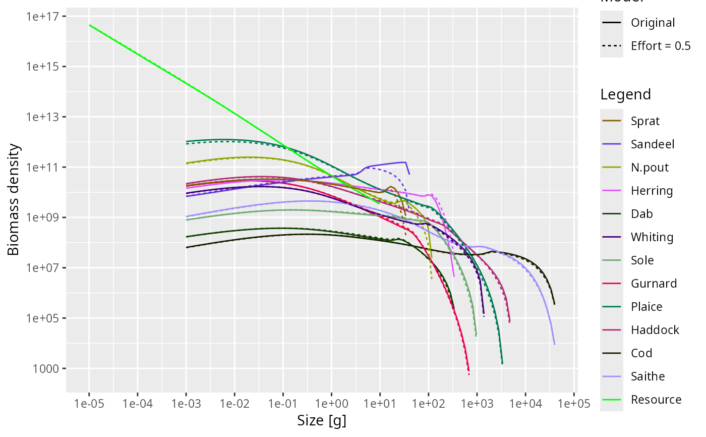
plotSpectra2() compares the abundance spectra from two MizerParams or MizerSim objects in a single plot. Colours identify species or groups and linetype identifies the object.

Usage

plotSpectra2(
  object1,
  object2,
  name1 = "First",
  name2 = "Second",
  power = 1,
  log_x = TRUE,
  log_y = TRUE,
  log = NULL,
  ...
)

plotlySpectra2(
  object1,
  object2,
  name1 = "First",
  name2 = "Second",
  power = 1,
  log_x = TRUE,
  log_y = TRUE,
  log = NULL,
  ...
)

Arguments

object1

First MizerParams or MizerSim object.

object2

Second MizerParams or MizerSim object.

name1, name2

Labels for the two objects, used in the linetype legend.

power

The abundance is plotted as the number density times the weight raised to power. The default power = 1 gives the biomass density, whereas power = 2 gives the biomass density with respect to logarithmic size bins.

log_x

If TRUE (default), use a log10 x-axis.

log_y

If TRUE (default), use a log10 y-axis.

log

Character string specifying which axes should use log10 scales, in the same form as the base plot() argument. For example, "x", "y", "xy" or "". If supplied, this overrides log_x and log_y.

...

Arguments passed to plotSpectra() for preparing the spectra data, for example species, time_range, wlim, ylim, resource, background or total.

Value

A ggplot2 object.

plotlySpectra2() returns a plotly object.

See also

Other plotting functions: addPlot(), animate.ArrayTimeBySpeciesBySize(), plot, plot2(), plotBiomass(), plotCDF(), plotCDF2(), plotDiet(), plotFMort(), plotFeedingLevel(), plotGrowthCurves(), plotMizerParams, plotMizerSim, plotPredMort(), plotRelative(), plotSpectra(), plotSpectraRelative(), plotYield(), plotYieldGear(), plotting_functions

Examples

# \donttest{
sim1 <- project(NS_params, t_max = 10, progress_bar = FALSE)
sim2 <- project(NS_params, effort = 0.5, t_max = 10, progress_bar = FALSE)
plotSpectra2(sim1, sim2, "Original", "Effort = 0.5")

# }