Plot abundance and biomass spectra

plotSpectra() plots the number density multiplied by a power of the weight, with the power specified by the power argument. When called with a MizerSim object, the abundance is averaged over the specified time range (a single value for the time range can be used to plot a single time step). When called with a MizerParams object the initial abundance is plotted.

Usage

plotSpectra(
  object,
  species = NULL,
  wlim = c(NA, NA),
  llim = c(NA, NA),
  ylim = c(NA, NA),
  power = 1,
  biomass = TRUE,
  total = FALSE,
  resource = TRUE,
  background = TRUE,
  highlight = NULL,
  log_x = TRUE,
  log_y = TRUE,
  log = NULL,
  size_axis = c("w", "l"),
  return_data = FALSE,
  ...
)

Arguments

object

An object of class MizerSim or MizerParams.

species

The species to be selected. Optional. By default all target species are selected. A vector of species names, or a numeric vector with the species indices, or a logical vector indicating for each species whether it is to be selected (TRUE) or not.

wlim

A numeric vector of length two providing lower and upper limits for the w axis. Use NA for the default: the lower default is min(params@w) / 100 when resource = TRUE (to show some resource below the fish grid) or min(params@w) when resource = FALSE; the upper default is max(params@w_full). Data is filtered to this range and the axis limits are set accordingly.

llim

A numeric vector of length two providing lower and upper limits for the length axis when size_axis = "l". Use NA to auto-scale to the data range. Data is filtered to this range and the axis limits are set accordingly.

ylim

A numeric vector of length two providing lower and upper limits for the y axis. Use NA to auto-scale to the data range. Values below 1e-20 are always filtered out from the data regardless of ylim[1]. Data above ylim[2] is filtered and the upper axis limit is set accordingly.

power

The abundance is plotted as the number density times the weight raised to power. The default power = 1 gives the biomass density, whereas power = 2 gives the biomass density with respect to logarithmic size bins.

biomass

Only used if power argument is missing. Then biomass = TRUE is equivalent to power=1 and biomass = FALSE is equivalent to power=0

total

A boolean value that determines whether the total over all species in the system is plotted as well. Note that even if the plot only shows a selection of species, the total is including all species. Default is FALSE.

resource

A boolean value that determines whether resource is included. Default is TRUE.

background

A boolean value that determines whether background species are included. Ignored if the model does not contain background species. Default is TRUE.

highlight

Name or vector of names of the species to be highlighted by being plotted with thicker lines.

log_x

If TRUE (default), use a log10 x-axis.

log_y

If TRUE (default), use a log10 y-axis.

log

Character string specifying which axes should use log10 scales, in the same form as the base plot() argument. For example, "x", "y", "xy" or "". If supplied, this overrides log_x and log_y.

size_axis

Whether to plot size as weight ("w", default) or length ("l"), using the allometric weight-length relationship.

return_data

A boolean value that determines whether the formatted data used for the plot is returned instead of the plot itself. Default value is FALSE

...

Further arguments used by only some of the methods:

For MizerSim methods:

• time_range: The time range (either a vector of values, a vector of min and max time, or a single value) to average the abundances over. Default is the final time step.

• geometric_mean: If TRUE then the average of the abundances over the time range is a geometric mean instead of the default arithmetic mean.

Value

A ggplot2 object, unless return_data = TRUE, in which case a data frame with the four variables 'w' (or 'l' if size_axis = "l"), 'value', 'Species', 'Legend' is returned. plotlySpectra() returns a plotly object.

Details

plotlySpectra() is the interactive plotly version. To compare spectra from two objects use plotSpectra2(). To show relative differences use plotSpectraRelative().

See also

plotting_functions

Other plotting functions: addPlot(), animate.ArrayTimeBySpeciesBySize(), plot, plot2(), plotBiomass(), plotCDF(), plotCDF2(), plotDiet(), plotFMort(), plotFeedingLevel(), plotGrowthCurves(), plotMizerParams, plotMizerSim, plotPredMort(), plotRelative(), plotSpectra2(), plotSpectraRelative(), plotYield(), plotYieldGear(), plotting_functions

Examples

# \donttest{
params <-  NS_params
sim <- project(params, effort=1, t_max=20, t_save = 2, progress_bar = FALSE)
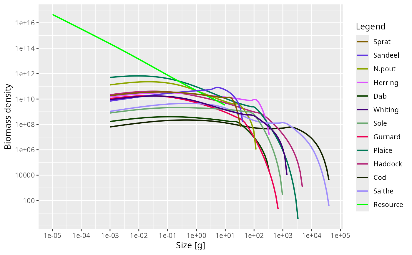
plotSpectra(sim)

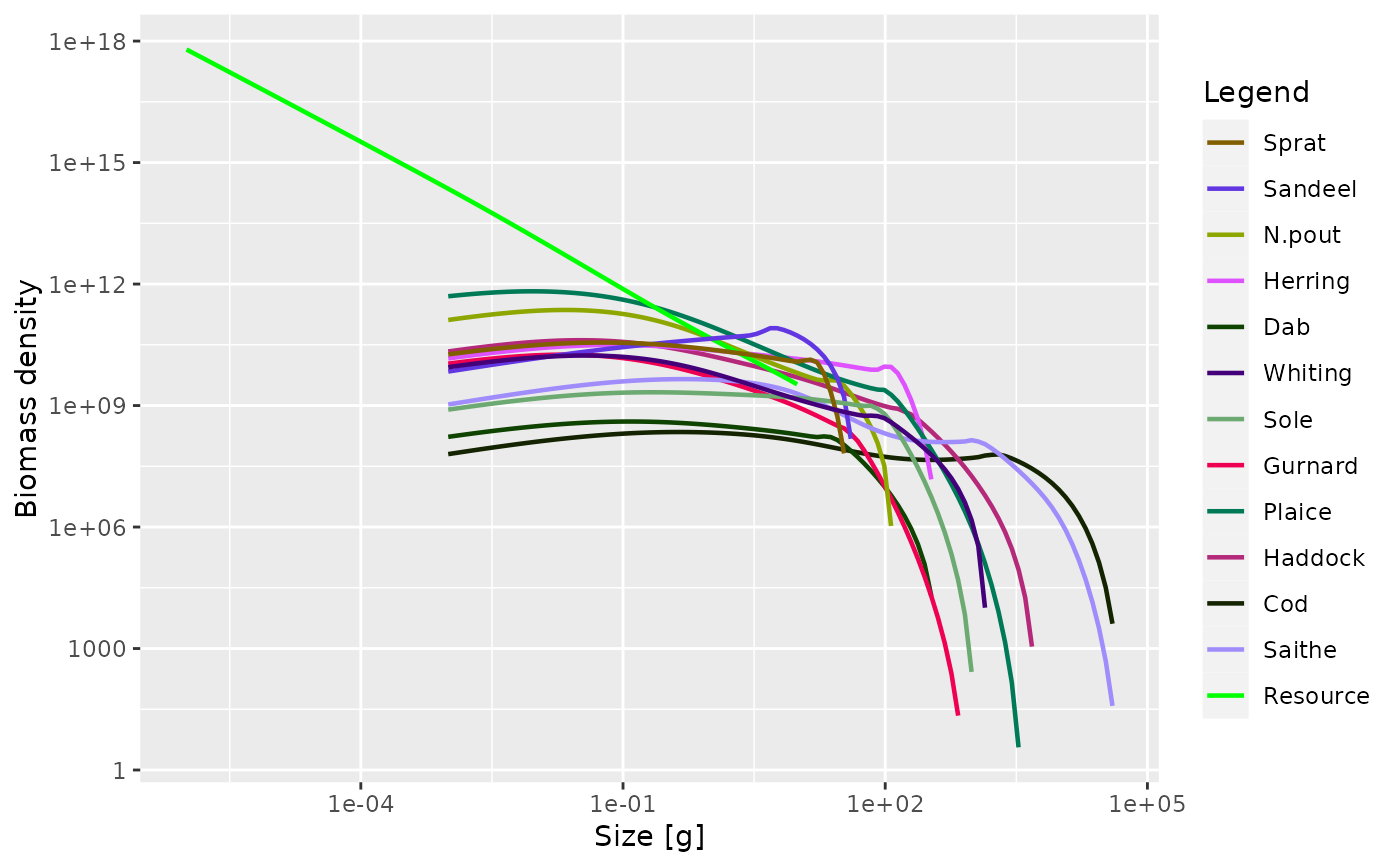
plotSpectra(sim, wlim = c(1e-6, NA))

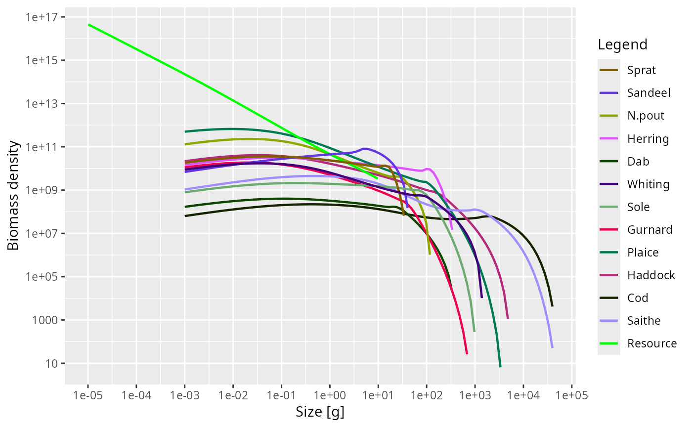
plotSpectra(sim, time_range = 10:20)

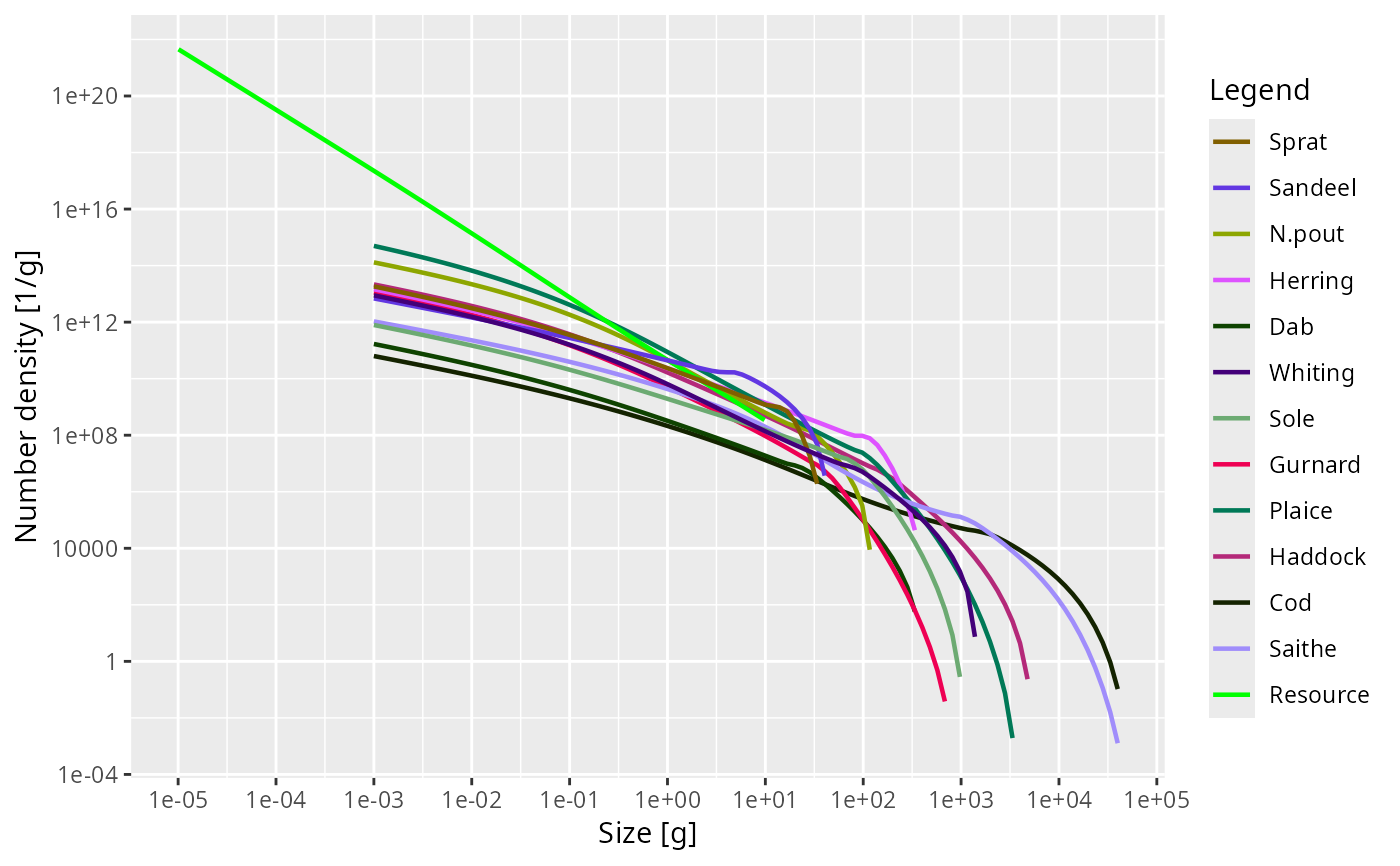
plotSpectra(sim, time_range = 10:20, power = 0)

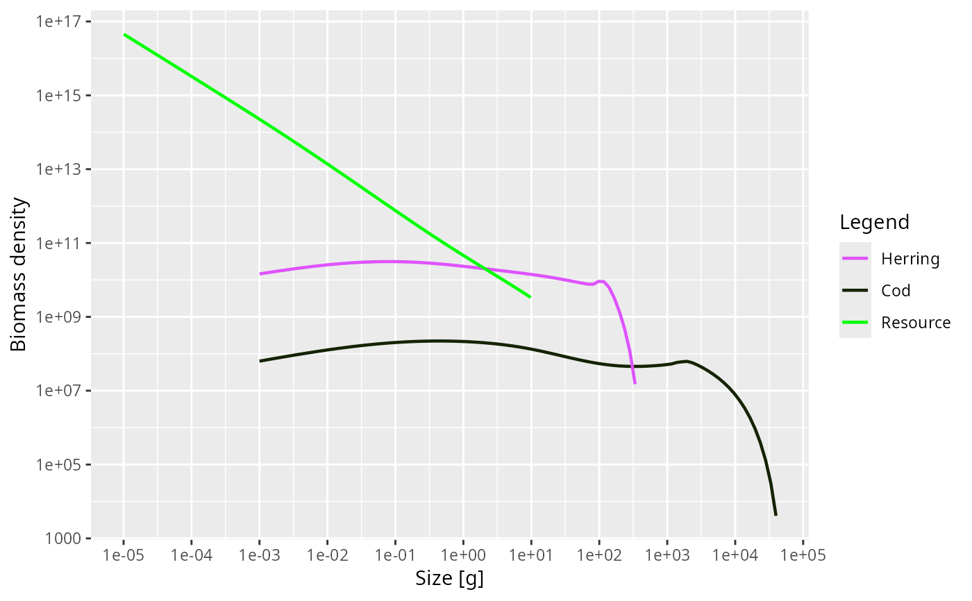
plotSpectra(sim, species = c("Cod", "Herring"), power = 1)

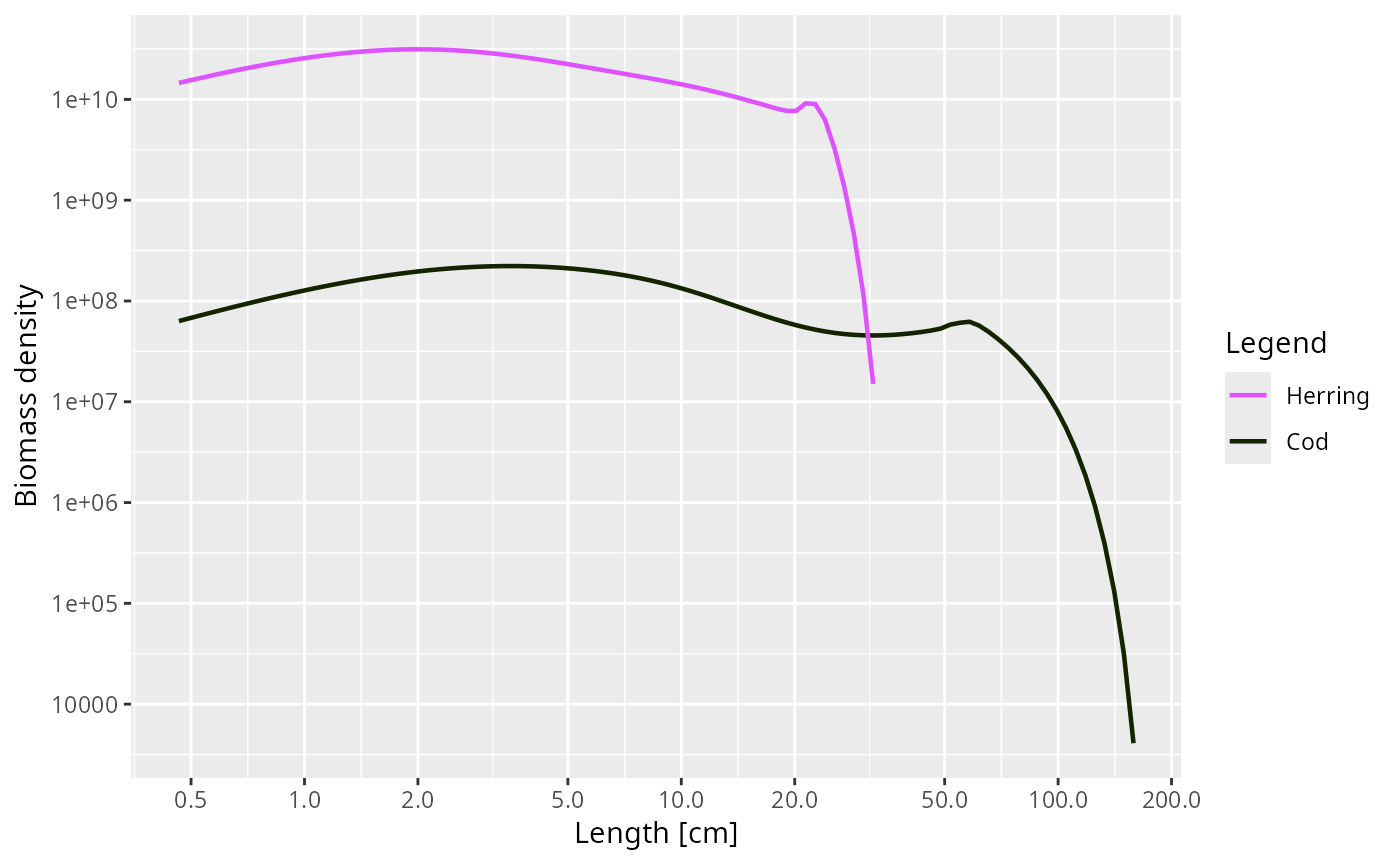
plotSpectra(sim, species = c("Cod", "Herring"), size_axis = "l")


# Returning the data frame
fr <- plotSpectra(sim, return_data = TRUE)
str(fr)
#> 'data.frame':	1024 obs. of  4 variables:
#>  $ w              : num  0.001 0.001 0.001 0.001 0.001 0.001 0.001 0.001 0.001 0.001 ...
#>  $ Biomass density: num  1.83e+10 6.92e+09 1.30e+11 1.46e+10 1.69e+08 ...
#>  $ Species        : chr  "Sprat" "Sandeel" "N.pout" "Herring" ...
#>  $ Legend         : chr  "Sprat" "Sandeel" "N.pout" "Herring" ...
# }