How far a model is from its steady state

Returns the rate at which the abundances would change if the model were projected forward from its current initial state, relative to those abundances. At a steady state this is zero, so it answers the question that every calibration workflow otherwise has to remember to ask: is this model still at its steady state?

Usage

getSteadyResidual(params, effort = params@initial_effort, dt = 1e-04)

Arguments

params: A MizerParams object.
effort: The fishing effort at which to evaluate the residual. By default the initial effort stored in params, which is the effort the model's steady state belongs to.
dt: The step length used for the resource and other components, whose dynamics functions are only available as one-step maps. Smaller is more accurate. Not used for the consumers, whose rate is exact.

Value

An ArraySpeciesBySize object (species x size) of per-capita rates of change in 1/year, NA where the density is zero. It carries two further attributes:

resource: The per-capita rate of change of the resource, a numeric vector over w_full, NA where the resource density is zero.
other: A named list with one entry per other component, holding its per-capita rate of change, or NA for a component whose state is not numeric.

Details

The value is a per-capita rate of change, in units of 1/year: $$R_i(w) = \frac{1}{N_i(w)}\frac{dN_i(w)}{dt}.$$ A value of 1e-8 means nothing is moving. A value of 0.05 means that size class would change by about 5% over the first year of a projection, and -0.05 that it would shrink by about that much. The sign is therefore the direction the model would drift.

For the consumers this is exact, not a finite-difference approximation: the backward-Euler transport coefficients used by project() satisfy $A N - S = -dt\,dN/dt$ identically, so evaluating them at dt = 1 gives the instantaneous rate with no time-discretisation error. The resource and other components have arbitrary user-supplied dynamics functions, so their rates are obtained by taking one short step of length dt, accurate to $O(dt)$.

Everything is evaluated at the model's own stored state — initialN(), initialNResource(), initialNOther() — using the model's own reproduction function and its own resource_dynamics. Nothing is substituted or held fixed. The number therefore answers exactly "if I called project() now, would anything move?", which is why it works for every model rather than only for the semichemostat resource that steadyNewton() requires.

Reading the result

The returned array is an ArraySpeciesBySize object, so it prints, summarises and plots itself:

res <- getSteadyResidual(params)
summary(res)                  # per-species minimum, mean and maximum
plot(res)                     # which species, and at which sizes

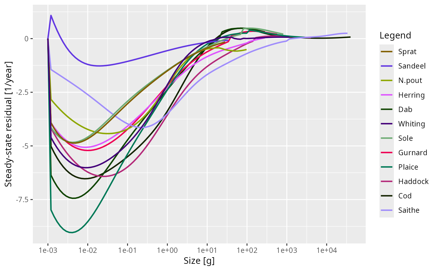
The plot is the diagnostic one: a model that is off steady state is usually off in one species, or one part of the size range, and the plot says which.

Size classes with no fish in them carry no information about steadiness — the relative rate of change of a zero density is undefined — so they are returned as NA. Use na.rm = TRUE in any summary, as the examples above do.

Do not reduce this to its maximum

max(abs(res)) is a tempting single-number verdict and a misleading one. The per-capita rate of a single size class is dominated by the fastest-relaxing cells, and near the egg size those turn over in hours: a model settled for every practical purpose can carry a cell rate of $10^4$/year there while nothing observable moves. Under the second-order scheme (see second_order_w()) this is severe enough to reverse the ordering between a converged model and one that has just been knocked off its steady state.

What mizer's own checks — the summary() line, and project(check_steady = TRUE) — judge instead is the relative rate of change of each species' biomass, which weights each size class by the mass it holds, and is the drift the user would actually see in plotBiomass(). Use this array to find out where a model is unsteady, and those checks to find out whether it is.

Examples

summary(getSteadyResidual(NS_params))
#> Steady-state residual [1/year] 
#> 12 species x 100 sizes
#> 
#>  Species         Min          Mean        Max
#>    Sprat -0.32010387  0.0014932474 0.01010982
#>  Sandeel -0.54637042 -0.0057605610 0.01148404
#>   N.pout -0.77251244  0.0065228584 0.03400740
#>  Herring -0.17077775  0.0019195590 0.02414716
#>      Dab -0.78476050 -0.0005368299 0.01726561
#>  Whiting -0.68433745  0.0024537842 0.02278352
#>     Sole -0.55536026 -0.0009899767 0.01048570
#>  Gurnard -0.04784682  0.0091143308 0.01765771
#>   Plaice -0.25831571  0.0065772666 0.02037855
#>  Haddock -0.84155214  0.0038039116 0.02842493
#>      Cod -1.23640575 -0.0047555940 0.01977439
#>   Saithe -0.84979728 -0.0040508052 0.01096811
# \donttest{
# Matching biomasses moves the model off its steady state, and the plot
# shows which species and which sizes have moved.
params <- NS_params
species_params(params)$biomass_observed <-
    c(0.8, 61, 12, 35, 1.6, 20, 10, 7.6, 135, 60, 30, 78)
species_params(params)$biomass_cutoff <- 10
params <- calibrateBiomass(params)
params <- matchBiomasses(params)
#> `matchBiomasses()` has rescaled the model and so moved it off its steady state. Run `steady()` to settle it again. You can check with `getSteadyResidual()`.
plot(getSteadyResidual(params))

# }