Find the steady state of a model

Puts the model onto a steady state of its own dynamics, changing no parameter: the reproduction rate, the resource and the consumer spectra all settle together at whatever the parameters you already have imply.

Usage

findSteadyState(
  params,
  solver = c("project", "newton"),
  effort = params@initial_effort,
  info_level = default_info_level(),
  ...
)

Arguments

params

A MizerParams object

solver

The solver to use: "project" to run the dynamics until they settle, "newton" to solve the steady-state equation directly. See Choosing a solver.

effort

The fishing effort to use throughout. By default the initial effort stored in params.

info_level

Controls the amount of information messages that are shown. Higher levels lead to more messages, info_level = 0 gives silence. The default is taken from the mizer_info_level option, see default_info_level().

...

Arguments for the chosen solver.

With solver = "project": distance_func, t_max, t_check, dt, distance_tol, residual_tol, amplitude_tol, amp_rel_tol, extinction_threshold, progress_bar and method, all as described in projectUntilSettled(). There is no t_save, because no trajectory is returned.

With solver = "newton": extinction_floor (default 1e-6), the relative abundance below which a species counts as extinct, plus solver_tol, maxit, jacobian, global and verbose as described in tuneSteadyState().

Value

A MizerParams object with the initial state replaced by the steady state found and no parameter changed. It carries a "convergence" attribute describing the solution found; see projectUntilSettled().

Details

This is the counterpart of tuneSteadyState(), which instead holds the reproduction rate and the resource at the values you supplied and adjusts erepro/R_max and cc_pp to make those values steady. Use this function when the parameters are the thing you want to keep — when asking what state a given model settles into, for instance under a changed fishing effort — and tuneSteadyState() while calibrating.

Nothing being held fixed means the search has more ways to end badly. With solver = "project" the run can settle on a limit cycle or drive a species extinct rather than reach a fixed point, and with either solver reproduction can collapse. Check the "convergence" attribute rather than assuming a fixed point was reached; see the section below.

Choosing a solver

solver = "project" (the default) runs the dynamics until they settle, via projectUntilSettled(), and takes the final state. It is exactly that function with the trajectory thrown away; call projectUntilSettled() instead if you want to watch the approach.

solver = "newton" solves the steady-state equation directly with a Newton-type root finder from the nleqslv package, so it converges even when the steady state is dynamically unstable, where the time-stepping solver diverges away from it. This is the natural entry point for a stability analysis with getStability().

The Newton solver treats the resource densities as unknowns alongside the fish and appends the resource steady-state equation to the system, so the resource density and the feeding levels it implies are self-consistent even where consumers are satiated. That equation is written for the default semichemostat resource dynamics, so solver = "newton" stops with an error for any other resource_dynamics; use solver = "project" there.

The Newton iteration also needs the residual \(F(N)\) to be continuous. A custom rate function registered with setRateFunction() that jumps as a function of the abundances makes \(F\) discontinuous, and where the equilibrium lies on the switching threshold there is no root at all, because neither branch is in equilibrium there. The solver then stalls (nleqslv termination code 3) and returns an iterate pinned to the threshold. See Discontinuous rate functions.

It also respects the active transport scheme: if the experimental second-order scheme is enabled (see second_order_w()) it solves the steady-state equation of that scheme. With the van Leer reconstruction the residual is only Lipschitz, so the iteration converges to a fixed point of the dynamics but not to machine precision. The unlimited "centred" reconstruction admits an undamped odd-even mode at a steady state with no physical diffusion, giving an ill-conditioned steady-state Jacobian for which the solver is not expected to converge.

What you get back may not be a steady state

The stopping criterion is a proxy. It says that two states t_per years apart differ by less than distance_tol on whatever scale the criterion is measured on; it does not say that the state reached is a fixed point. There are four ways the returned object can fail to be one:

the run converged on its own scale while the biomasses are still visibly drifting (termination = "distance_tolerance");
the run reached t_max without converging (termination = "time_limit");
the run settled on a limit cycle (termination = "cycle_detected"), in which case the state stored is one point on that cycle;
the run stopped because a species was going extinct (termination = "extinction").

So treat the result as a claim to be checked rather than as a guarantee:

attr(params, "convergence")$attractor  # "fixed_point", "limit_cycle" or NA
attr(params, "convergence")$residual   # largest biomass drift, in 1/year
isSteady(params)                       # TRUE if within tolerance
summary(params)                        # includes the biomass-drift verdict
plot(getSteadyResidual(params))        # which species, and at which sizes

attractor is the field that answers the question: it is "fixed_point" only where the measured biomass drift is within residual_tol, so it cannot be satisfied by a distance function that has merely gone quiet. termination says how the run ended and converged whether the solver met its own criterion; neither is a claim about the state. The last line says where the model is not steady, which is the one to reach for when it is not: a model that is off steady state is usually off in one species or one part of the size range, and the plot names it. See getSteadyResidual() for why the verdict is phrased in terms of biomass drift rather than the largest per-capita rate.

The messages this function prints say the same thing — a converged run whose biomasses are still moving reports the drift and adds "Reduce the tolerance on the distance function to converge further." — but they are suppressed by info_level = 0, so in a script the "convergence" attribute is the reliable check.

Finally, a genuine fixed point need not be a stable one. Use getStability() to find out, and solver = "newton" to converge onto a fixed point that the dynamics themselves would run away from.

Examples

# \donttest{
params <- findSteadyState(NS_params, solver = "newton")
#> The biomasses of the solution change at up to 6e-07 per year.
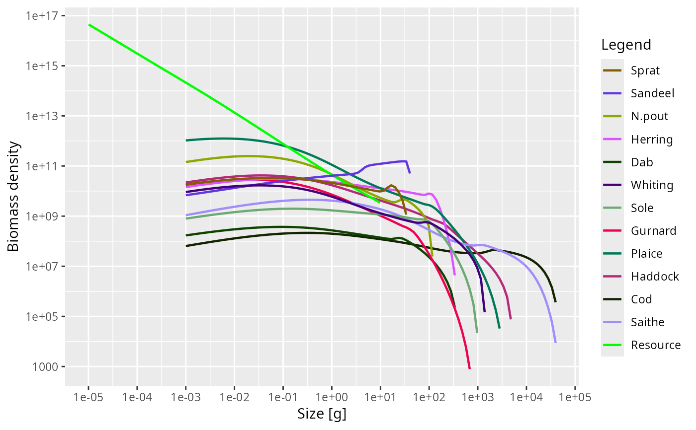
plotSpectra(params)

# }