Tune a model so that the state it is in becomes a steady state

Solves for the consumer size spectra while holding the reproduction rate (RDD), the resource and any other components at the values stored in params, and then adjusts the parameters that generate those held values so that they are steady too. This is the function to use while setting up and calibrating a model: holding the inputs to the fish dynamics fixed is what makes the search reliable.

Usage

tuneSteadyState(
  params,
  solver = c("project", "newton"),
  effort = params@initial_effort,
  preserve = c("reproduction_level", "erepro", "R_max"),
  info_level = default_info_level(),
  ...
)

Arguments

params

A MizerParams object

solver

The solver to use: "project" to run the dynamics until they settle, "newton" to solve the steady-state equation directly. See Choosing a solver.

effort

The fishing effort to use throughout. By default the initial effort stored in params.

preserve

Specifies whether the reproduction_level should be preserved (default) or the maximum reproduction rate R_max or the reproductive efficiency erepro. See setBevertonHolt() for an explanation of the reproduction_level.

info_level

Controls the amount of information messages that are shown. Higher levels lead to more messages, info_level = 0 gives silence. The default is taken from the mizer_info_level option, see default_info_level().

...

Arguments for the chosen solver.

With solver = "project": t_max, t_check, dt, distance_tol, residual_tol, amplitude_tol, amp_rel_tol, extinction_threshold, progress_bar and method, all as described in projectUntilSettled(). There is no t_save, because no trajectory is returned. Note that distance_tol here defaults to 0.1 * dt and measures the largest relative change in egg production, because the distance function is distanceMaxRelRDI(). residual_tol is judged on the model as the search sees it, with reproduction, the resource and the other components pinned; the residual reported in the result is measured again on the model that is actually returned.

With solver = "newton": solver_tol (default 1e-6), a tolerance on the per-capita rate of change passed to nleqslv::nleqslv(). It was called residual_tol before mizer 3.3, a name that now belongs to the biomass drift criterion above; maxit (default 200); jacobian, either "update" (default, the Jacobian is computed once and then updated cheaply each iteration — nleqslv's "Broyden") or "recompute" (a numerical Jacobian at every iteration — nleqslv's "Newton"); global, the globalisation strategy (default "dbldog", a robust double-dogleg trust region); and verbose to trace the iterations.

Value

A MizerParams object with the initial state replaced by the steady state found, and with erepro/R_max and cc_pp adjusted as described above. It carries a "convergence" attribute describing the solution found; see projectUntilSettled(). Check it: convergence is not guaranteed.

Details

Concretely, three things are held fixed during the search and two parameters are re-derived afterwards:

The reproduction rate is pinned at getRDD(params). Afterwards, if the model uses Beverton-Holt reproduction, setBevertonHolt() restores the density dependence so that it reproduces exactly that rate at the new spectra. Use preserve to say which of the reproduction parameters should be kept as it was.
The resource abundance is held at initialNResource(params). Afterwards the resource capacity cc_pp is recomputed so that this abundance is a steady state of the resource under the new spectra. If the capacity had been set by hand (frozen), it is rebalanced and thereby unfrozen.
Other components are held constant throughout and are not adjusted.

So the model you get back is at a fixed point of the full dynamics, with reproduction and the resource free, and getStability() can be applied to it directly. Contrast findSteadyState(), which changes no parameter and instead lets the reproduction rate and the resource move to wherever the parameters you already have put them.

Holding those inputs fixed is what makes the search reliable, but it does not make the result certain: the state that is stored is only as close to a fixed point as the solver's tolerance allowed, and with solver = "project" the run may instead have stopped on a limit cycle or on a species going extinct. Check the result rather than assuming it; see the section below.

Choosing a solver

solver = "project" (the default) runs the dynamics until they settle, via projectUntilSettled(), using distanceMaxRelRDI() as its distance function. It needs no extra packages and works with any resource dynamics.

solver = "newton" solves the steady-state equation directly with a Newton-type root finder from the nleqslv package. It converges even when the steady state is dynamically unstable, where the time-stepping solver cannot, and it discovers the support of the steady state automatically. It starts from the spectra in initialN(params), so a reasonable initial guess still matters — for example the spectra from a nearby stable parameterisation, or the (diverging) output of solver = "project".

Because the resource is held fixed either way, solver = "newton" here does not need the resource to be a semichemostat, unlike in findSteadyState() where the resource is one of the unknowns.

What you get back may not be a steady state

The stopping criterion is a proxy. It says that two states t_per years apart differ by less than distance_tol on whatever scale the criterion is measured on; it does not say that the state reached is a fixed point. There are four ways the returned object can fail to be one:

the run converged on its own scale while the biomasses are still visibly drifting (termination = "distance_tolerance");
the run reached t_max without converging (termination = "time_limit");
the run settled on a limit cycle (termination = "cycle_detected"), in which case the state stored is one point on that cycle;
the run stopped because a species was going extinct (termination = "extinction").

So treat the result as a claim to be checked rather than as a guarantee:

attr(params, "convergence")$attractor  # "fixed_point", "limit_cycle" or NA
attr(params, "convergence")$residual   # largest biomass drift, in 1/year
isSteady(params)                       # TRUE if within tolerance
summary(params)                        # includes the biomass-drift verdict
plot(getSteadyResidual(params))        # which species, and at which sizes

attractor is the field that answers the question: it is "fixed_point" only where the measured biomass drift is within residual_tol, so it cannot be satisfied by a distance function that has merely gone quiet. termination says how the run ended and converged whether the solver met its own criterion; neither is a claim about the state. The last line says where the model is not steady, which is the one to reach for when it is not: a model that is off steady state is usually off in one species or one part of the size range, and the plot names it. See getSteadyResidual() for why the verdict is phrased in terms of biomass drift rather than the largest per-capita rate.

The messages this function prints say the same thing — a converged run whose biomasses are still moving reports the drift and adds "Reduce the tolerance on the distance function to converge further." — but they are suppressed by info_level = 0, so in a script the "convergence" attribute is the reliable check.

Finally, a genuine fixed point need not be a stable one. Use getStability() to find out, and solver = "newton" to converge onto a fixed point that the dynamics themselves would run away from.

Examples

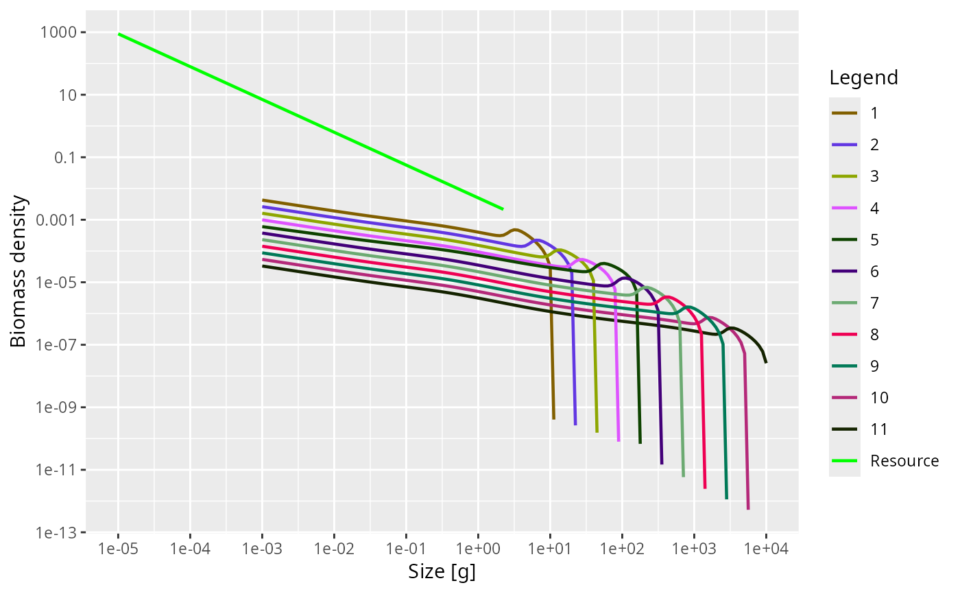
# \donttest{
params <- newTraitParams()
species_params(params)$gamma[5] <- 3000
params <- tuneSteadyState(params)
#> Reached the convergence tolerance after 12 years. The biomasses change at up to 0.0025 per year.
plotSpectra(params)

# }