Scan a model over a range of values

Varies one aspect of a model over a range of values and measures a quantity at each of them. At every value the model is projected until it settles onto an attractor, and the quantity is measured on that attractor rather than at whatever state the projection happened to stop at.

Usage

scanModel(
  params,
  scan_values,
  set_func,
  value_func = getBiomass,
  species = NULL,
  scan_name = NULL,
  scan_units = NULL,
  value_name = NULL,
  value_units = NULL,
  reference_lines = NULL,
  current_scan_value = NULL,
  continuation = TRUE,
  distance_func = distanceSSLogN,
  distance_tol = 0.001,
  residual_tol = steady_residual_tol(),
  t_check = 15 * dt,
  t_max = 100,
  dt = 0.1,
  amplitude_tol = 0.01,
  amp_rel_tol = 0.1,
  extinction_threshold = 1e-06,
  method = c("euler", "predictor_corrector", "tr_bdf2"),
  t_sample = 10,
  sample_all = FALSE,
  progress_bar = interactive(),
  info_level = 0,
  ...
)

Arguments

params: An object of class MizerParams.
scan_values: A numeric vector of values to scan over.
set_func: A function of (params, value) returning a modified MizerParams object. Several are provided: scanEffort(), scanFishingMortality() and scanSpeciesParam().
value_func: A function of a MizerSim returning the quantity to measure. Defaults to getBiomass().
species: The species to keep in the result. By default all of the series that value_func returns.
scan_name: A string naming the quantity that is varied, used for the x-axis label and as the name of the first column of the result. Taken from set_func when it supplies one.
scan_units: A string giving the units of that quantity.
value_name: A string naming the quantity that is measured, used for the y-axis label and as the name of the second column of the result. Taken from what value_func returns when it supplies one.
value_units: A string giving the units of that quantity.
reference_lines: An optional named numeric vector of positions on the x axis for plot.MizerScan() to mark with vertical dashed lines, for example c(F_MSY = 0.32). Taken from set_func when it supplies one.
current_scan_value: The value at which the model currently sits. When given, the scan works outwards from it in both directions so that every projection starts from a neighbouring attractor rather than from a distant state, and each of the two directions begins again at the model as it was given. Pass "auto" to ask set_func for it. By default the values are scanned in the order given, which is also how you trace a hysteresis branch deliberately: pass a decreasing scan_values.
continuation: Whether each scan value should start from the attractor reached at the previous one. Default TRUE.
distance_func: A function that will be called at every convergence check with both the previous and the new state and that should return a number measuring the distance between them. See distanceSSLogN().
distance_tol: The projection at each scan value stops once the number returned by distance_func for two states t_check years apart drops below distance_tol. The default is tighter than the one projectUntilSettled() uses on its own, because a scan produces a curve, and a loosely converged point does not average away: it shows up as a kink in the curve and as spurious width in the band. Loosen it to go faster, and use the residual column of the result to check whether that cost you anything.
residual_tol: The largest relative rate of biomass change, in 1/year, at which a scan point may still be recorded as a fixed point. See projectUntilSettled(). A point that meets distance_tol but not this is not sampled as a single value, which would draw it as a band of zero width.
t_check: The interval in years at which convergence is checked, see projectUntilSettled(). Must be a positive multiple of dt; the default 15 * dt is an odd multiple, which is what lets a period-2 cycle be seen.
t_max: The longest time to project at each scan value.
dt: The time step to use.
amplitude_tol: The minimum relative biomass amplitude for a persistent oscillation to count as a limit cycle rather than a fixed point.
amp_rel_tol: Maximum relative change of amplitude between successive periods for a cycle to count as settled.
extinction_threshold: A species is treated as going extinct once its reproduction rate falls below this fraction of its value at the start of the projection.
method: The numerical method to use, see project().
t_sample: The number of years over which to average when the model has settled onto neither a fixed point nor a limit cycle.
sample_all: Whether to run the sampling projection even at a fixed point, where it is not otherwise needed. Set this if value_func needs more than one time step.
progress_bar: Whether to show a text progress bar over the scan values.
info_level: Controls how much the projections say for themselves. Defaults to 0, because a scan makes one projection per scan value and summarises them itself; raise it when investigating why one of them behaved oddly.
...: Further arguments are passed on to distance_func.

Value

An object of class MizerScan, which is a data frame with one row per scan value and series, carrying the metadata that plot() needs.

Details

You say what to vary by giving a function that changes the model, and what to measure by giving a function that computes a quantity from a simulation. So a yield-versus-fishing-mortality curve, a bifurcation diagram over fishing effort and a scan over the resource carrying capacity are all the same function call with different arguments.

This is a generic function with a method for objects of class MizerParams.

What is measured, and where

At each scan value the model is projected with projectUntilSettled(), which stops as soon as it recognises that the model has settled onto a fixed point or onto a limit cycle, and reports which of the two happened. What happens next depends on that answer:

A fixed point: The state does not change, so there is nothing to average. The quantity is read off the settled state with no further projection at all, and the reported minimum and maximum are equal to it.
A limit cycle: The model is projected for exactly one period of the detected cycle and the quantity is averaged over it, which is its long-term average. The minimum and maximum over the cycle are reported too.
Neither: The model did not settle within t_max years, or a species went extinct. The quantity is averaged over the last t_sample years and the scan values concerned are named in a message, because those points should not be relied on.

Averaging over exactly one period is both faster and more accurate than averaging over a fixed number of years. A window that is not a whole number of periods leaves a residue of the oscillation in the average, which shows up as a jagged curve. The window is rounded to a whole number of time steps, so it can differ from the true period by up to dt/2; if you need the average more accurately, reduce dt rather than lengthening the window, because a longer window that is not a whole number of periods is worse, not better.

Writing the two functions

set_func(params, value) takes a MizerParams object and one entry of scan_values and returns a modified MizerParams. It must be idempotent — set_func(set_func(p, v), v) must give the same thing as set_func(p, v) — because with continuation = TRUE it is applied to the object it returned at the previous scan value. Setting something is idempotent; appending something is not, so a function that adds a gear must check whether the gear is already there. See scanFishingMortality() for a worked example.

There is no effort argument, because there does not need to be one: project() and projectUntilSettled() both take the fishing effort from params@initial_effort, so a set_func() that changes the effort is all it takes to scan over effort, and a scan over something else never has to mention fishing at all.

value_func(sim) takes a MizerSim and returns either a time by series matrix, as getBiomass(), getYield(), getSSB(), getN() and sizeIntegral() all do, or a plain numeric vector over time, as getMeanWeight() does. When it returns a matrix carrying value_name and units attributes — which all of mizer's MizerSim methods do — those are used for the y-axis label unless you override them.

Note that at a fixed point value_func() is handed a simulation with a single time step, so a function that needs more than one time step will not work there. Set sample_all = TRUE to force the sampling projection at every scan value.

Neither function can be given extra arguments through ..., which is reserved for distance_func. Use a closure instead, for example value_func = function(sim) getBiomass(sim, min_w = 10).

Examples

# \donttest{
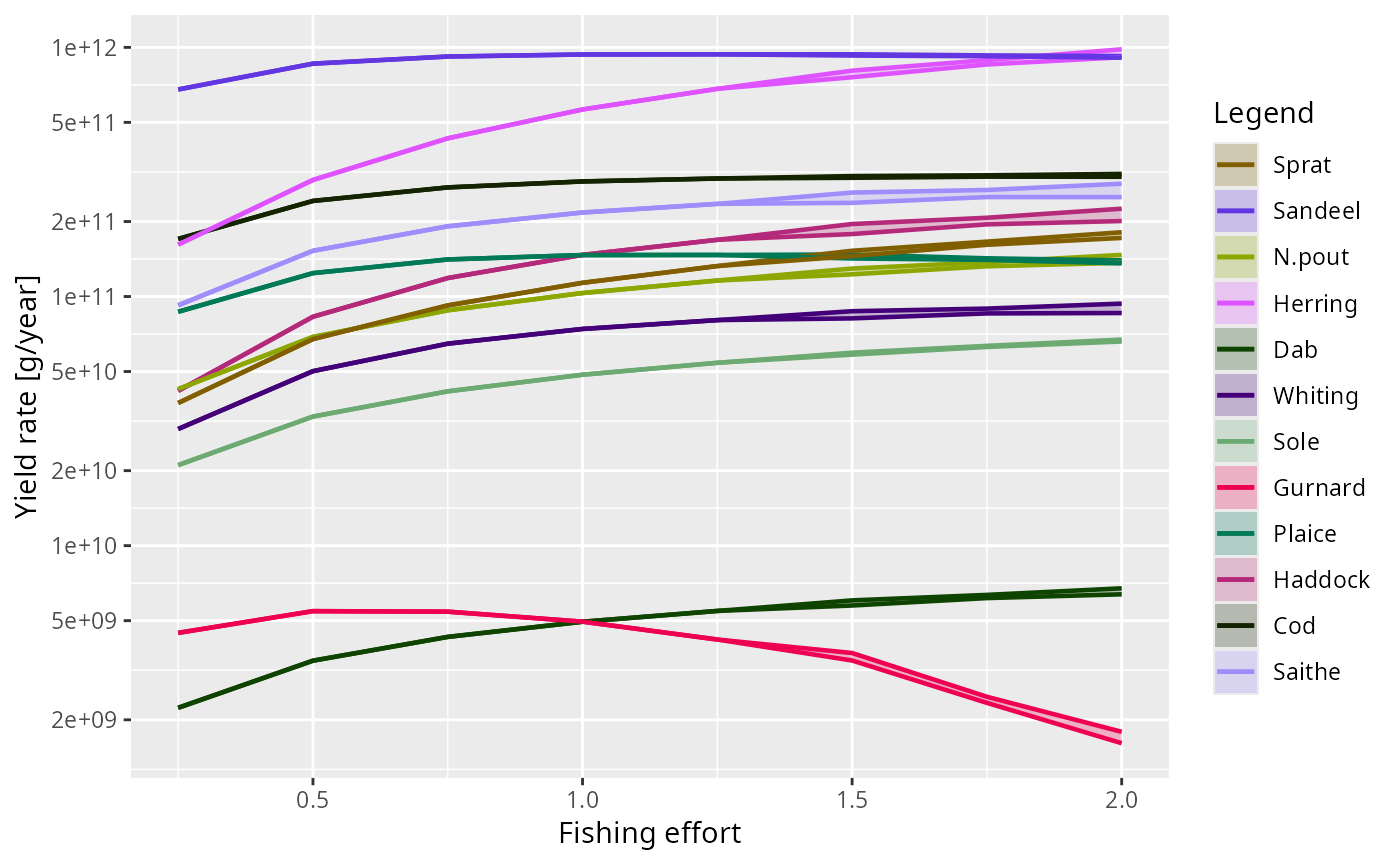
# A bifurcation diagram over fishing effort
scan <- scanModel(NS_params, scan_values = seq(0, 2, 0.25),
                  set_func = scanEffort(), value_func = getYield)
#> The model settled onto a limit cycle at Fishing effort = 1.5, 1.75, 2. The value there is the average over one period of the cycle.
plot(scan, style = "envelope")


# A yield curve for a single species, and the F at which it is largest
cod <- scanModel(NS_params, scan_values = seq(0, 1.2, 0.2),
                 set_func = scanFishingMortality("Cod"),
                 value_func = getYield, species = "Cod")
plot(cod, mark_max = TRUE, log_y = FALSE)

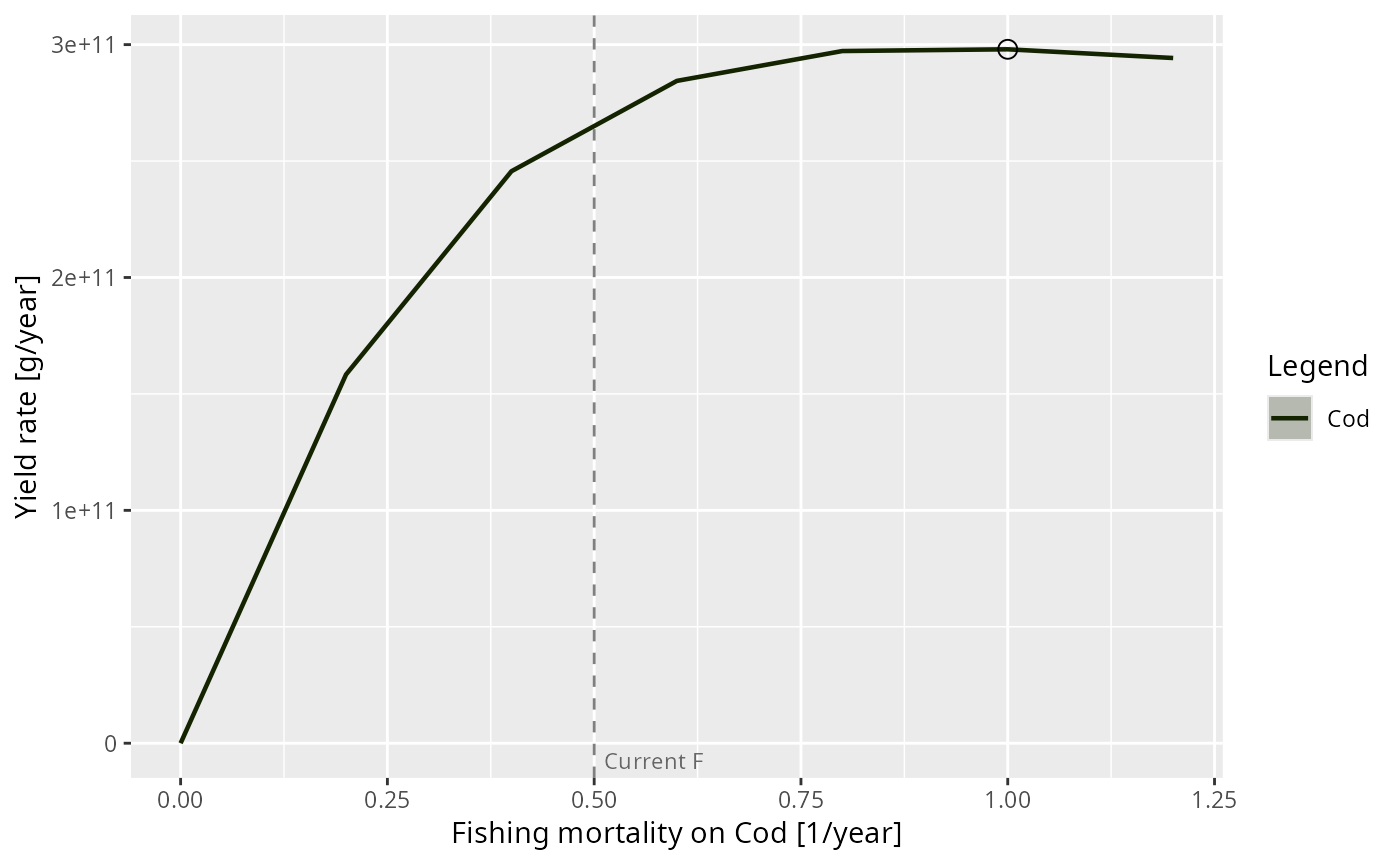attr(cod, "at_max")
#> Cod 
#>   1 

# Scanning something that has nothing to do with fishing
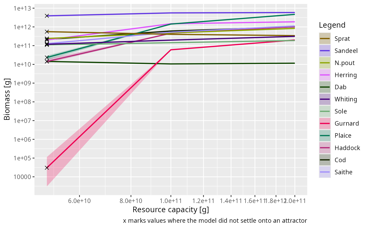
kappa <- resource_params(NS_params)$kappa
plot(scanModel(NS_params, scan_values = kappa * c(0.5, 1, 2),
               set_func = function(params, value) {
                   resource_params(params)$kappa <- value
                   params
               },
               scan_name = "Resource capacity", scan_units = "g"),
     log_x = TRUE)
#> Warning: Gurnard are going extinct.
#> A species was on its way to extinction at Resource capacity = 5e+10, which stopped the projection early. The value there is only the average over the 10 years following that point.

# }