Find a steady state by directly solving the steady-state equation

This is an alternative to steady() that finds the steady state by solving the steady-state equation F(N) = 0 with a Newton-type root finder instead of running the dynamics to convergence. The advantage is that it converges to the steady state even when that steady state is dynamically unstable, a case in which steady() fails because the time-stepping diverges away from the fixed point.

Usage

steadyNewton(params, ...)

# S3 method for class 'MizerParams'
steadyNewton(
  params,
  effort = params@initial_effort,
  preserve = c("reproduction_level", "erepro", "R_max"),
  reproduction = c("fixed", "dynamic"),
  extinction_floor = 1e-06,
  verbose = FALSE,
  tol = 1e-06,
  maxit = 200,
  method = c("Broyden", "Newton"),
  global = "dbldog",
  info_level = default_info_level(),
  ...
)

Arguments

params: A MizerParams object. Its initial_n is used as the starting guess for the iteration.
...: Unused.
effort: The fishing effort. By default the initial effort stored in params.
preserve: Specifies whether the reproduction_level should be preserved (default) or the maximum reproduction rate R_max or the reproductive efficiency erepro. See setBevertonHolt() for an explanation of the reproduction_level. This argument is ignored when reproduction = "dynamic".
reproduction: If "fixed", the reproduction rate (RDD) is held constant at the initial value. If "dynamic", the reproduction dynamics are run dynamically and the reproduction parameters are not adjusted. Default is "fixed".
extinction_floor: The relative abundance floor below which a species is considered extinct. Only used when reproduction = "dynamic". Default is 1e-6.
verbose: If TRUE then the solver iterations will be traced and printed to the console. Default is FALSE.
tol: Convergence tolerance passed to nleqslv::nleqslv() (both the function-value tolerance ftol and the step tolerance xtol).
maxit: Maximum number of iterations for nleqslv::nleqslv().
method: The nleqslv::nleqslv() method, either "Newton" (with a numerical Jacobian calculated at each iteration) or "Broyden" (which calculates the full Jacobian only once and then only updates it on each
global: The globalisation strategy passed to nleqslv::nleqslv(). The default "dbldog" (double dogleg) is a robust trust-region method.
info_level: Controls the amount of information messages and warnings that are shown. Higher levels lead to more messages, info_level = 0 gives silence. The default is taken from the mizer_info_level option, see default_info_level().

Value

A MizerParams object with the initial state set to the steady state.

Details

By default, or when reproduction = "fixed", the function holds the reproduction rate (RDD) constant while solving for the consumer spectra, substitutes the analytic steady state of the resource, and keeps any other components constant. After the spectra have been found it restores density-dependent Beverton-Holt reproduction with setBevertonHolt(), honouring the preserve argument exactly as steady() does. If reproduction = "dynamic", the reproduction dynamics are run dynamically, meaning the reproduction rate varies during the solve and the reproduction parameters are not adjusted.

The consumer densities are solved for in log space, which both keeps them positive and conditions the otherwise badly-scaled system. The unknowns are the size classes in the full potential grid support (running from the egg size up to the grid truncation limit support_top_idx()), regardless of whether they carry non-zero density in the supplied initial spectra. A smoothed log-abundance penalty floor is applied to all size classes, which automatically handles zero-density and tail classes smoothly and prevents singular Jacobians. After convergence, size classes that remain at or near the floor are set to zero. This allows the solver to automatically discover the support of the steady state. The nonlinear system is solved with a globalised Newton iteration from the nleqslv package, starting from the current initial_n. Newton's method converges from any starting point in the root's basin of attraction (which is unrelated to the dynamic stability of the steady state), so a reasonable initial guess should still be supplied in initialN(params) — for example the spectra from a nearby stable parameterisation, or the (diverging) output of steady().

The solver respects the active transport scheme: if the experimental second-order scheme is enabled (see second_order_w()) it solves the steady-state equation of that scheme. With the van Leer reconstruction the residual is only Lipschitz, so the iteration converges to a fixed point of the dynamics but not to machine precision. The unlimited "centred" reconstruction admits an undamped odd-even mode at a steady state with no physical diffusion, giving an ill-conditioned steady-state Jacobian for which the solver is not expected to converge.

The Newton iteration also needs the residual \(F(N)\) to be continuous. A custom rate function registered with setRateFunction() that jumps as a function of the abundances makes \(F\) discontinuous, and where the equilibrium lies on the switching threshold there is no root at all, because neither branch is in equilibrium there. The solver then stalls (nleqslv termination code 3) and returns an iterate pinned to the threshold. See Discontinuous rate functions.

Only the default semichemostat resource dynamics (resource_dynamics = "resource_semichemostat") are currently supported, because the solver substitutes the analytic resource steady state. For other resource dynamics the function stops with an error.

Examples

# \donttest{
params <- steadyNewton(NS_params)
#> The biomasses of the solution change at up to 7.7e-07 per year.
#> Warning: The following species require an unrealistic value greater than 1 for `erepro`: Sprat
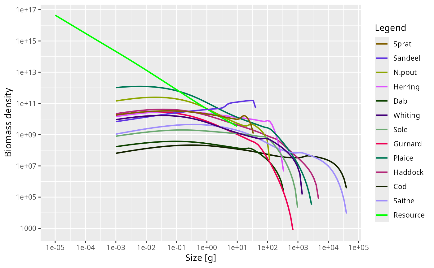
plotSpectra(params)

# }